2.1.PLOT()AND ALLIED FUNCTIONS 11 The existing parameter settings are stored in oldpar,so that they can be restored later.Margins are reduced in size (mar rep(2,4))so that each margin has room for two lines of text only.The figure area will take in the exact r-and y-limits (xaxs="i",yaxs="i"),rather than extending slightly beyond those limits.The margin parameters are set so that labels will be printed 1.5 lines out from the margin,tick labels 0.75 lines out from the margin,and ticks right on the margin. Here are some of the more common settings: -Plotting symbols:pch (choice of symbol);cex ("character expansion");col (color).Thus par(cex=1.2)increases the plot symbol size 20%above the default. Lines:Ity (line type);lwd (line width);col(color). Axis limits:xlim;ylim.(Assuming xaxs="r",x-axis limits are by default extended by 4% relative to the data limits.Specify xaxs="i"to make the default an exact fit to the data limits. For the y-axis,replace xaxs by yaxs and x by y.) Axis annotation and labels:cex.axis (character expansion for axis annotation,independently of cex);cex.labels(size of the axis labels);mgp(margin line for the axis title,axis labels,and axis line;default is mgp=c(3,1,0)). -Graph margins:mar (inner margins,clockwise from the bottom;the out of the box default is mar=c(5.1,4.1,4.1,2.1),in lines out from the axis);oma (outer margins,relevant when there are multiple graphs on the one graphics page). -Plot shape:pty="s"gives a square plot(must be set using par()). Multiple graphs on the one graphics page:Specify par(mfrow=c(m,n))to get an m rows by n columns layout of graphs on a page. Type help(par)to get a(very extensive)complete list. In most (not all)instances,the change can be made either in a call to a plotting function (eg, plot(),points()),or using par().If made in a call to a plotting function,the change applies only to that call.If made using par(),changes remain in place until changed again,or until a new device is opened. 2.1.2 Adding points,lines and text-examples Here is a simple example (Figure 2.2)that uses the function text()to label the points on a plot. Figure 2.2:Plot of brain weight against body weight,for selected primates. ●Human @ #Data used in plot primates DAAG package ●Chimp Bodywt Brainwt ●Gorilla Potar monkey 10.0 Rhesus monkey 115 Potar monkey Gorilla 207.0 406 Human 62.0 1320 050100 200 Rhesus monkey 6.8 179 Body weight(kg) Chimp 52.2 440 Code that gives the above plot is:
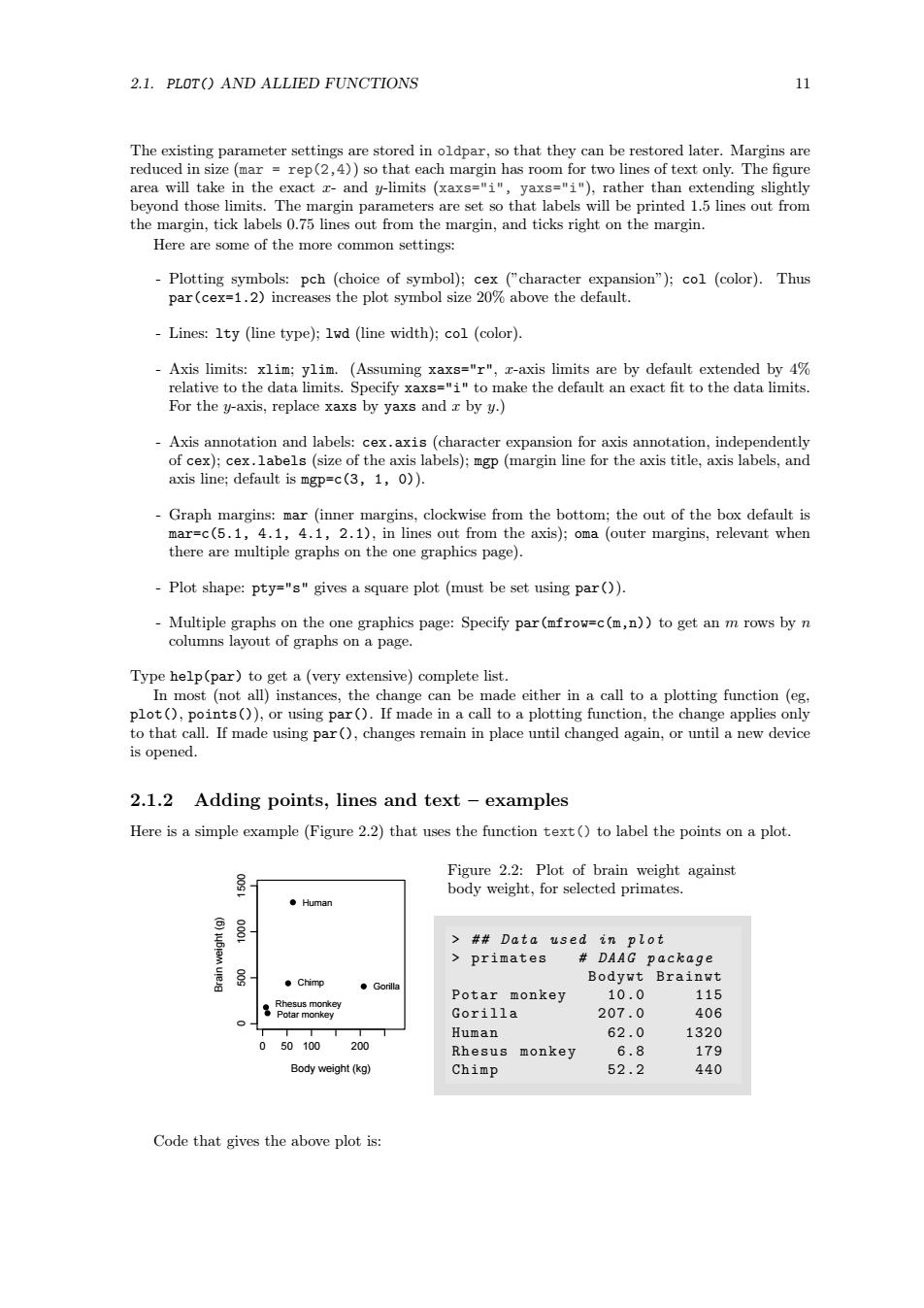
2.1. PLOT() AND ALLIED FUNCTIONS 11 The existing parameter settings are stored in oldpar, so that they can be restored later. Margins are reduced in size (mar = rep(2,4)) so that each margin has room for two lines of text only. The figure area will take in the exact x- and y-limits (xaxs="i", yaxs="i"), rather than extending slightly beyond those limits. The margin parameters are set so that labels will be printed 1.5 lines out from the margin, tick labels 0.75 lines out from the margin, and ticks right on the margin. Here are some of the more common settings: - Plotting symbols: pch (choice of symbol); cex (”character expansion”); col (color). Thus par(cex=1.2) increases the plot symbol size 20% above the default. - Lines: lty (line type); lwd (line width); col (color). - Axis limits: xlim; ylim. (Assuming xaxs="r", x-axis limits are by default extended by 4% relative to the data limits. Specify xaxs="i" to make the default an exact fit to the data limits. For the y-axis, replace xaxs by yaxs and x by y.) - Axis annotation and labels: cex.axis (character expansion for axis annotation, independently of cex); cex.labels (size of the axis labels); mgp (margin line for the axis title, axis labels, and axis line; default is mgp=c(3, 1, 0)). - Graph margins: mar (inner margins, clockwise from the bottom; the out of the box default is mar=c(5.1, 4.1, 4.1, 2.1), in lines out from the axis); oma (outer margins, relevant when there are multiple graphs on the one graphics page). - Plot shape: pty="s" gives a square plot (must be set using par()). - Multiple graphs on the one graphics page: Specify par(mfrow=c(m,n)) to get an m rows by n columns layout of graphs on a page. Type help(par) to get a (very extensive) complete list. In most (not all) instances, the change can be made either in a call to a plotting function (eg, plot(), points()), or using par(). If made in a call to a plotting function, the change applies only to that call. If made using par(), changes remain in place until changed again, or until a new device is opened. 2.1.2 Adding points, lines and text – examples Here is a simple example (Figure 2.2) that uses the function text() to label the points on a plot. ● ● ● ● ● 0 50 100 200 0 500 1000 1500 Body weight (kg) Brain weight (g) Potar monkey Gorilla Human Rhesus monkey Chimp Figure 2.2: Plot of brain weight against body weight, for selected primates. > # # Data used in plot > primates # DAAG package Bodywt Brainwt Potar monkey 10.0 115 Gorilla 207.0 406 Human 62.0 1320 Rhesus monkey 6.8 179 Chimp 52.2 440 Code that gives the above plot is:
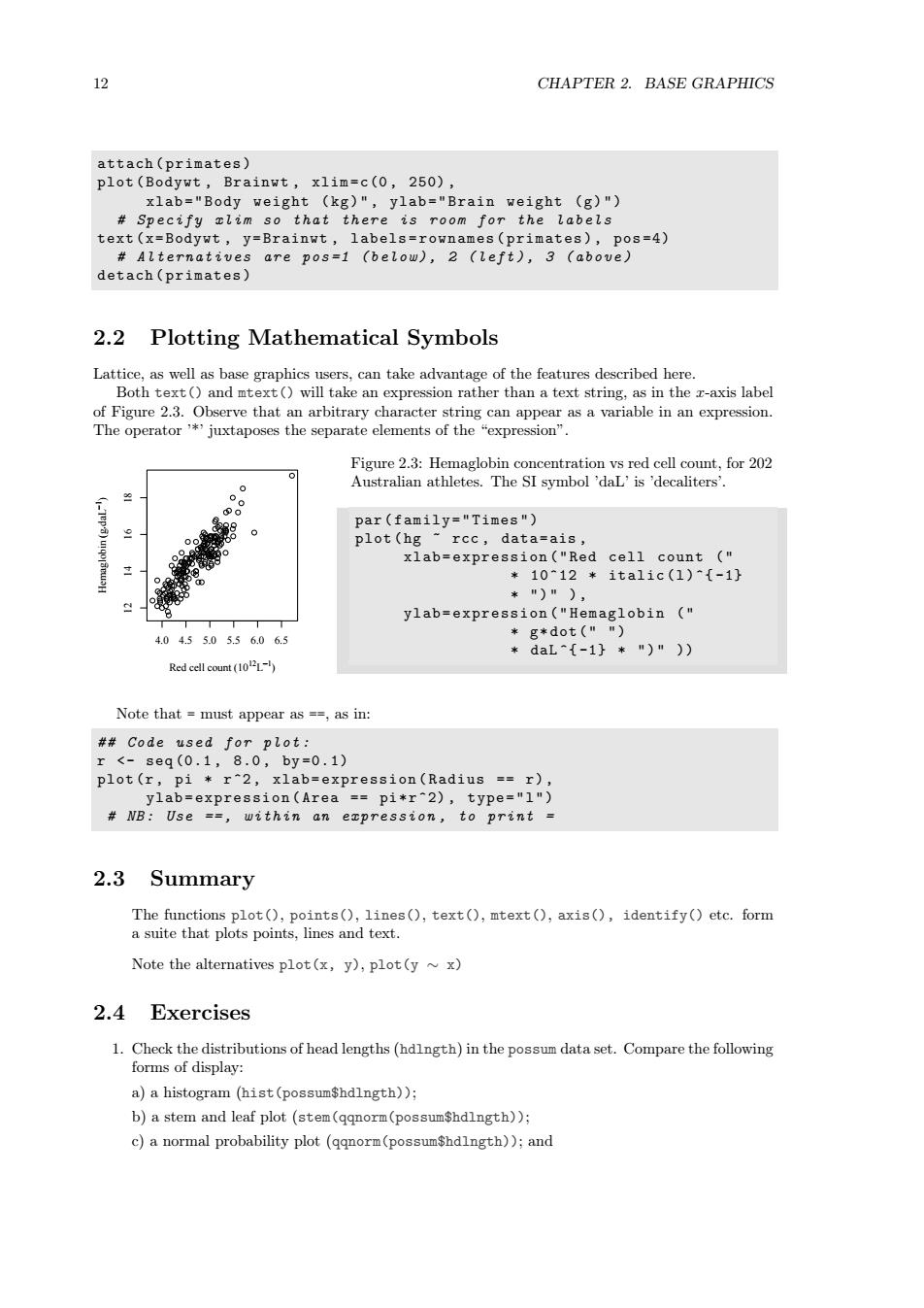
12 CHAPTER 2.BASE GRAPHICS attach(primates) plot(Bodywt,Brainwt,xlim=c(0,250), xlab="Body weight (kg)",ylab="Brain weight (g)") Specify xlim so that there is room for the labels text(x=Bodywt,y=Brainwt,labels=rownames(primates),pos=4) Alternatives are pos=1 (below),2 (left),3 (above) detach(primates) 2.2 Plotting Mathematical Symbols Lattice,as well as base graphics users,can take advantage of the features described here. Both text()and mtext()will take an expression rather than a text string,as in the r-axis label of Figure 2.3.Observe that an arbitrary character string can appear as a variable in an expression. The operator'*juxtaposes the separate elements of the "expression". Figure 2.3:Hemaglobin concentration vs red cell count,for 202 Australian athletes.The SI symbol 'daL'is 'decaliters' par(family="Times") plot (hg rcc,data=ais, xlab=expression("Red cell count ( *1012*ita1ic(1)^[-1] *")"), ylab=expression("Hemaglobin ( 4.04.55.05.56.06.5 *g*dot("") *daL[-1]*")n)) Red cell count (10L-) Note that must appear as ==as in: #Code used for plot: r<-seg(0.1,8.0,by=0.1) plot(r,pi r2,xlab=expression(Radius =r), ylab=expression(Area ==pi*r2),type="1") NB:Use ==within an expression,to print 2.3 Summary The functions plot(),points(),lines(),text(),mtext(),axis(),identify()etc.form a suite that plots points,lines and text. Note the alternatives plot(x,y),plot(y ~x) 2.4 Exercises 1.Check the distributions of head lengths(hdlngth)in the possum data set.Compare the following forms of display: a)a histogram (hist (possum$hdlngth)); b)a stem and leaf plot (stem(qqnorm(possum$hdlngth)); c)a normal probability plot (qqnorm(possum$hdlngth));and
12 CHAPTER 2. BASE GRAPHICS attach ( primates ) plot ( Bodywt , Brainwt , xlim = c (0 , 250) , xlab = " Body weight ( kg ) " , ylab = " Brain weight ( g ) " ) # Specify xlim so that there is room for the labels text ( x = Bodywt , y = Brainwt , labels = rownames ( primates ) , pos =4) # Alternatives are pos =1 ( below ) , 2 ( left ) , 3 ( above ) detach ( primates ) 2.2 Plotting Mathematical Symbols Lattice, as well as base graphics users, can take advantage of the features described here. Both text() and mtext() will take an expression rather than a text string, as in the x-axis label of Figure 2.3. Observe that an arbitrary character string can appear as a variable in an expression. The operator ’*’ juxtaposes the separate elements of the “expression”. ● ● ● ● ● ● ● ●● ● ● ● ●● ● ● ● ● ● ● ● ● ● ● ● ● ● ● ● ● ●● ● ● ● ● ● ● ● ● ● ● ● ● ● ● ● ● ● ●● ● ●● ●● ● ● ●● ● ●●● ● ● ● ● ● ● ● ● ● ● ● ● ● ● ● ● ● ● ● ● ● ● ● ● ● ● ● ● ● ● ● ● ● ● ● ● ● ● ● ● ● ● ● ● ● ● ● ● ● ● ● ● ● ● ● ● ● ● ● ● ● ● ● ● ●● ● ● ● ● ● ● ●● ● ● ● ● ● ● ● ● ● ●● ● ● ● ● ● ● ● ● ● ● ● ● ● ● ● ● ● ● ● ●● ● ● ● ● ● ● ● ● ● ●● ● ● ● ● ● ● ● ● ● ● ● ● ● ● ● ● ● ● 4.0 4.5 5.0 5.5 6.0 6.5 12 14 16 18 Red cell count (1012L−1 ) Hemaglobin (g d⋅ aL−1 ) Figure 2.3: Hemaglobin concentration vs red cell count, for 202 Australian athletes. The SI symbol ’daL’ is ’decaliters’. par ( family = " Times " ) plot ( hg ~ rcc , data = ais , xlab = expression ( " Red cell count ( " * 10^12 * italic ( l )^{ -1} * " ) " ) , ylab = expression ( " Hemaglobin ( " * g * dot ( " " ) * daL ^{ -1} * " ) " )) Note that = must appear as ==, as in: # # Code used for plot : r <- seq (0.1 , 8.0 , by =0.1) plot (r , pi * r ^2 , xlab = expression ( Radius == r ) , ylab = expression ( Area == pi * r ^2) , type = " l " ) # NB : Use == , within an expression , to print = 2.3 Summary The functions plot(), points(), lines(), text(), mtext(), axis(), identify() etc. form a suite that plots points, lines and text. Note the alternatives plot(x, y), plot(y ∼ x) 2.4 Exercises 1. Check the distributions of head lengths (hdlngth) in the possum data set. Compare the following forms of display: a) a histogram (hist(possum$hdlngth)); b) a stem and leaf plot (stem(qqnorm(possum$hdlngth)); c) a normal probability plot (qqnorm(possum$hdlngth)); and