
6 CHAPTER 1.PRELIMINARIES A further package that will be discussed here,the ggplot?package,is not an R commander suggested package,and requires separate installation.Enter,at the command line: install("ggplot2",dependencies=TRUE) 1.2 The R Commander 1.3 The R Commander GUI The R commander gives a graphical user interface(GUI)to a wide range of abilities,in the base R system and in R packages.This includes graphical abilities,in the lattice and rgl packages as well as in base graphics. To start the R commander,start up R and enter:1 library(Rcmdr) This opens an R Commander script window,with the output window underneath.This window can be closed by clicking on the x in the top left corner.If thus closed,enter Commander()to reopen it again later in the session. The R Commander GUI-a guide to getting started Once the points that will now be noted are understood,use of the R Commander should for the most part be straightforward. From GUI to writing code:The R commander displays the code that it generates.Users can take this code,modify it,and re-run it.The code can be run either from the R Commander script window or from the R console window (if open). The active data set:The R commander has the notion of an active data set.Here are alternative ways to make a data set active.Start by clicking on the Data drop-down menu.Then Click on Active data set,and pick from among data sets,if any,in the workspace. Click on Import data,and follow instructions,to read in data from a file.The data set is read into the workspace,at the same time becoming the active data set. Click on New data set...,then entering data via a spreadsheet-like interface. Click on Data in packages,click on Read Data from Package,then identify one of the attached packages and choose a data set from among those that are included with the package. A further possibility is to load data from an R image(.RData)file;click on Load data set... Creating graphs:To draw graphs,click on the Graphs drop-down menu.Then Click on Scatterplot...to obtain a scatterplot.This uses the function scatterplot()from the car package,which is an option rich interface to functions that are in base graphics. .Click on X Y conditioning plot...for lattice scatterplots and panels of scatterplots. Click on 3D graph to obtain a 3D scatterplot,using the R Commander function scatter3d() that is an interface to functions in the rgl package. 1At startup,the R Commander checks whether all the suggested packages,needed to use all its features,are available. If some are missing,then upon starting up,the R commander offers to install them.For installing such packages,there must be a live internet connection
6 CHAPTER 1. PRELIMINARIES A further package that will be discussed here, the ggplot2 package, is not an R commander suggested package, and requires separate installation. Enter, at the command line: install ( " ggplot2 " , dependencies = TRUE ) 1.2 The R Commander 1.3 The R Commander GUI The R commander gives a graphical user interface (GUI) to a wide range of abilities, in the base R system and in R packages. This includes graphical abilities, in the lattice and rgl packages as well as in base graphics. To start the R commander, start up R and enter:1 library ( Rcmdr ) This opens an R Commander script window, with the output window underneath. This window can be closed by clicking on the × in the top left corner. If thus closed, enter Commander() to reopen it again later in the session. The R Commander GUI – a guide to getting started Once the points that will now be noted are understood, use of the R Commander should for the most part be straightforward. From GUI to writing code: The R commander displays the code that it generates. Users can take this code, modify it, and re-run it. The code can be run either from the R Commander script window or from the R console window (if open). The active data set: The R commander has the notion of an active data set. Here are alternative ways to make a data set active. Start by clicking on the Data drop-down menu. Then • Click on Active data set, and pick from among data sets, if any, in the workspace. • Click on Import data, and follow instructions, to read in data from a file. The data set is read into the workspace, at the same time becoming the active data set. • Click on New data set . . . , then entering data via a spreadsheet-like interface. • Click on Data in packages, click on Read Data from Package, then identify one of the attached packages and choose a data set from among those that are included with the package. • A further possibility is to load data from an R image (.RData) file; click on Load data set . . . Creating graphs: To draw graphs, click on the Graphs drop-down menu. Then • Click on Scatterplot . . . to obtain a scatterplot. This uses the function scatterplot() from the car package, which is an option rich interface to functions that are in base graphics. • Click on X Y conditioning plot . . . for lattice scatterplots and panels of scatterplots. • Click on 3D graph to obtain a 3D scatterplot, using the R Commander function scatter3d() that is an interface to functions in the rgl package. 1At startup, the R Commander checks whether all the suggested packages, needed to use all its features, are available. If some are missing, then upon starting up, the R commander offers to install them. For installing such packages, there must be a live internet connection

1.3.THE R COMMANDER GUI 7 Statistics(&fitting models):Click on the Statistics drop down menu to get submenus that give summary statistics and/or carry out various statistical tests.This includes(under Contingency tables) tables of counts and(under Means)One-way ANOVA.Also,click here to get access to the Fit models submenu. *Models:Click here to extract information from model objects once they have been fitted.(NB: To fit a model,go to the Statistics drop down menu,and click on Fit models)
1.3. THE R COMMANDER GUI 7 Statistics (& fitting models): Click on the Statistics drop down menu to get submenus that give summary statistics and/or carry out various statistical tests. This includes (under Contingency tables) tables of counts and (under Means) One-way ANOVA. Also, click here to get access to the Fit models submenu. *Models: Click here to extract information from model objects once they have been fitted. (NB: To fit a model, go to the Statistics drop down menu, and click on Fit models)

8 CHAPTER 1.PRELIMINARIES
8 CHAPTER 1. PRELIMINARIES
Chapter 2 Base Graphics Base Graphics implements a relatively "traditional"style of graphics: Plots go to one or more pages of a graphics device(screen,or hardcopy) plot(),etc. Sets up figure region,with user region inside,usually starts the graph. Other functions that initiate a graph include hist()and boxplot(). Typically,it also creates the main part,or all,of the graph. Use points(),lines(),text(),mtext(),axis(),rug(),identify(),etc., to add to the graph. Plot y vs x with(women,plot(height,weight))#0lder syntax plot(weight height,data=women)#Newer syntax (graphics formula) Caveat Some base graphics functions do not take a data parameter To see some of the possibilities that traditional(or base)R graphics offers,enter demo (graphics) Press the Enter key to move to each new graph. 2.1 plot()and allied functions Here are two examples. library(DAAG) attach(elasticband)R can now find distance stretch plot(distance ~stretch) plot(ACT year,data=austpop,type="1") plot(ACT-year,data-austpop,type="b") detach(elasticband) Figure 2.1 demonstrates some of the features of base graphics.Base graphics is highly flexible, but often requires a great deal of attention to detail.There are annoying inconsistencies. 2.1.1 Fine control-parameter settings Users who execute the code given above for Figure 2.1 will notice that the layout is different;there will be bigger margins,and the tick labels and the axis labels will be further out.To get the layout shown,there were some small changes to parameter settings: #Invoke once device is open,and before starting the plot oldpar <-par(mar =rep(2,4),xaxs="i",yaxs="i",mgp=c(1.5,0.75,0))
Chapter 2 Base Graphics Base Graphics implements a relatively “traditional” style of graphics: Plots go to one or more pages of a graphics device (screen, or hardcopy) plot(), etc. Sets up figure region, with user region inside, usually starts the graph. Other functions that initiate a graph include hist() and boxplot(). Typically, it also creates the main part, or all, of the graph. Use points(), lines(), text(), mtext(), axis(), rug(), identify(), etc., to add to the graph. Plot y vs x with(women, plot(height, weight)) # Older syntax plot(weight ∼ height, data=women) # Newer syntax (graphics formula) Caveat Some base graphics functions do not take a data parameter To see some of the possibilities that traditional (or base) R graphics offers, enter demo ( graphics ) Press the Enter key to move to each new graph. 2.1 plot() and allied functions Here are two examples. library ( DAAG ) attach ( elasticband ) # R can now find distance & stretch plot ( distance ~ stretch ) plot ( ACT ~ year , data = austpop , type = " l " ) plot ( ACT ~ year , data = austpop , type = " b " ) detach ( elasticband ) Figure 2.1 demonstrates some of the features of base graphics. Base graphics is highly flexible, but often requires a great deal of attention to detail. There are annoying inconsistencies. 2.1.1 Fine control – parameter settings Users who execute the code given above for Figure 2.1 will notice that the layout is different; there will be bigger margins, and the tick labels and the axis labels will be further out. To get the layout shown, there were some small changes to parameter settings: # # Invoke once device is open , and before starting the plot oldpar <- par ( mar = rep (2 ,4) , xaxs = " i " , yaxs = " i " , mgp = c (1.5 ,0.75 ,0)) 9

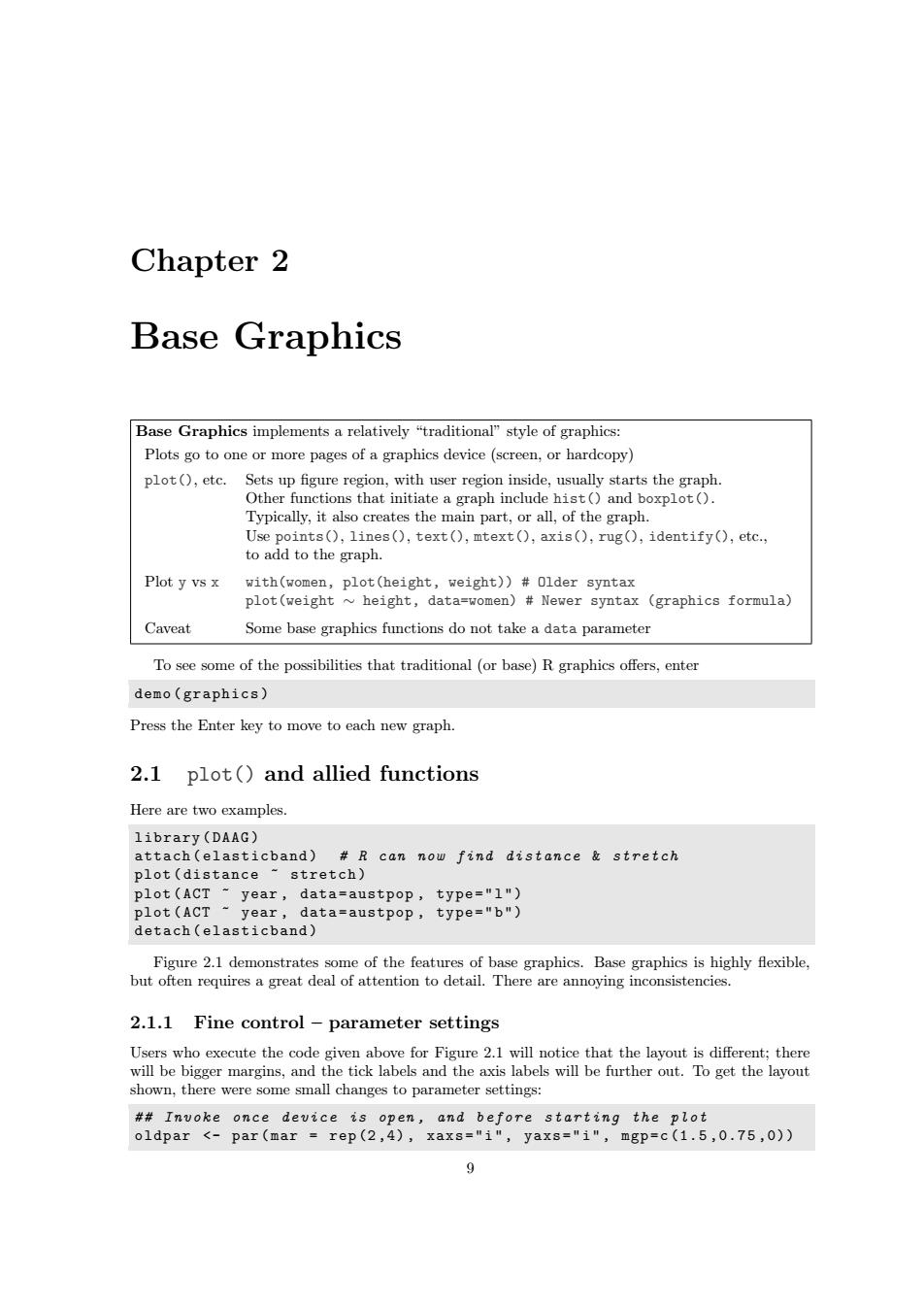
10 CHAPTER 2.BASE GRAPHICS Side 3 ##A:Set up plotting region,but(type="n")do not plot.Suppress axes axis labels plot(0~0,xlim=c(0,26.5),ylim=c(-0.05,34.25),xlab=M,ylab="",type="n",axes=FALSE) 男 ##B:Plot symbols 0-25.Overlay with numbers 0-25 grayscale <-gray(seq(from=0.1,by=0.05,length=13)) xpos <-seq(from=1,by=2,length=13);ypos <-rep(23,13);ypos2 <-ypos-2 points(ypos~xpos,cex=3,col=grayscale,pch=0:12) points(ypos2~xpos,cex=3,col=rev(grayscale),pch=13:25) text(ypos~xpos,labels=paste(0:12),cex=0.75) text(ypos2 ~xpos,labels=paste(13:25).cex=0.75) o ① 公+X⑥可☒米令 、2 -23 03 4 156位6002④ 2 ③A 啊 21 ##C:Enlarged and/or coloured symbols or text 18 Xp0s<-c(21.5,23.5,25.5):yp0s<-rep(18,3):yp0s2<-ypos-2 points(ypos~xpos,pch=0:2,cex=4:2,col=gray(c(.2,.4,.6))) text(ypos2 ~xpos,labels=letters[1:3],cex=2:4,col=gray(c(.2,.4,.6))) a 16 ##D:Positioning of label with respect to a point p0s<-c(22.5,21.5,22.5,23.5) above(3) yp0s<-c(10,11,12,11) ● 12 let(2)● ●ight(4) 11 points(ypos~xpos,pch=16,cex=1.5,col=gray((1:4)/5)) posText <-c("below (pos=1)","left(2)"."above (3)","right (4)") 10 below(pos=1) text(ypos~xpos,posText,pos=1:4) ##E:Sides (margins)are numbered 1,...4.Label them acordingly mtext(side=4,line=0.5,text="Side 4",adj=1)#Flush right on margin (Flush left:adj=0) ##Center labels in margins 1 to 3 for(i in 1:3)mtext(side=i,line=0.5,text=paste("Side",i)) #Label selected plotting positions 1abp0s<-c0,10:12,16,18,21,23) for(pos in labpos)axis(side=4,at=pos,las=2) 0 Side 1 Figure 2.1:Here are illustrated a number of features of traditional graphics plots.The code reproduces the points,labels,ticks,tick labels and axis labels,but not the printing of the code in the figure region
10 CHAPTER 2. BASE GRAPHICS ##A: Set up plotting region, but (type="n") do not plot. Suppress axes & axis labels plot(0 ~ 0, xlim=c(0, 26.5), ylim=c(−0.05, 34.25), xlab="", ylab="", type="n", axes=FALSE) ##B: Plot symbols 0 − 25. Overlay with numbers 0 − 25 ● ● grayscale <− gray(seq(from=0.1, by=0.05, length=13)) xpos <− seq(from=1, by=2, length=13); ypos <− rep(23,13); ypos2 <− ypos−2 points(ypos ~ xpos, cex=3, col=grayscale, pch=0:12) ● ● ● ● ● points(ypos2 ~ xpos, cex=3, col=rev(grayscale), pch=13:25) 0 1 2 3 4 5 6 7 8 9 10 11 12 13 14 15 16 17 18 19 20 21 22 23 24 25 text(ypos ~ xpos, labels=paste(0:12), cex=0.75) text(ypos2 ~ xpos, labels=paste(13:25), cex=0.75) ##C: Enlarged and/or coloured symbols or text xpos <− c(21.5, 23.5, 25.5); ypos <− rep(18, 3); ypos2 <− ypos−2 points(ypos ~ xpos, pch=0:2, cex=4:2, col=gray(c(.2, .4, .6))) ● text(ypos2 ~ xpos, labels=letters[1:3], cex=2:4, col=gray(c(.2, .4, .6))) a b c ##D: Positioning of label with respect to a point xpos <− c(22.5, 21.5, 22.5, 23.5) ypos <− c(10, 11, 12, 11) points(ypos ~ xpos, pch=16, cex=1.5, col=gray((1:4)/5)) ● ● ● ● posText <− c("below (pos=1)", "left (2)", "above (3)", "right (4)") below (pos=1) left (2) above (3) right (4) text(ypos ~ xpos, posText, pos=1:4) ##E: Sides (margins) are numbered 1, ...4. Label them acordingly Side 4 Side 1 Side 2 Side 3 mtext(side=4, line=0.5, text="Side 4", adj=1) # Flush right on margin (Flush left: adj=0) ## Center labels in margins 1 to 3 for (i in 1:3) mtext(side=i, line=0.5, text=paste("Side",i)) ## Label selected plotting positions labpos <− c(0, 10:12, 16, 18, 21, 23) for (pos in labpos) axis(side=4, at=pos, las=2) 0 10 11 12 16 18 21 23 Figure 2.1: Here are illustrated a number of features of traditional graphics plots. The code reproduces the points, labels, ticks, tick labels and axis labels, but not the printing of the code in the figure region