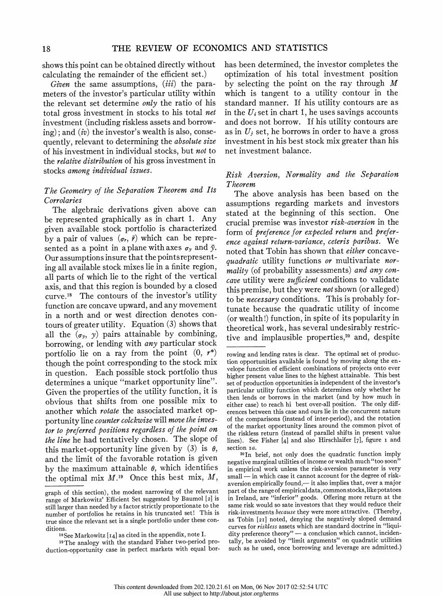
18 THE REVIEW OF ECONOMICS AND STATISTICS shows this point can be obtained directly without has been determined,the investor completes the calculating the remainder of the efficient set.)optimization of his total investment position Given the same assumptions,(iii)the para- by selecting the point on the ray through M meters of the investor's particular utility within which is tangent to a utility contour in the the relevant set determine only the ratio of his standard manner.If his utility contours are as total gross investment in stocks to his total net in the Ui set in chart 1,he uses savings accounts investment (including riskless assets and borrow-and does not borrow.If his utility contours are ing);and(i)the investor's wealth is also,conse-as in U;set,he borrows in order to have a gross quently,relevant to determining the absolute size investment in his best stock mix greater than his of his investment in individual stocks,but not to net investment balance. the relalive distribution of his gross investment in stocks among individual issues. Risk Aversion,Normality and the Separation Theorem The Geometry of the Separation Theorem and Its The above analysis has been based on the Corrolaries assumptions regarding markets and investors The algebraic derivations given above can stated at the beginning of this section.One be represented graphically as in chart 1.Any crucial premise was investor risk-aversion in the given available stock portfolio is characterized by a pair of values (ar,F)which can be repre- form of preference for expected return and prefer- sented as a point in a plane with axes ay and ence against relurn-variance,ceteris paribus.We noted that Tobin has shown that either concave- Our assumptions insure that the pointsrepresent- guadratic utility functions or multivariate nor- ing all available stock mixes lie in a finite region, all parts of which lie to the right of the vertical mality (of probability assessments)and any con- cave utility were sufficient conditions to validate axis,and that this region is bounded by a closed this premise,but they were not shown (or alleged) curve.18 The contours of the investor's utility to be necessary conditions.This is probably for- function are concave upward,and any movement tunate because the quadratic utility of income in a north and or west direction denotes con- (or wealth!)function,in spite of its popularity in tours of greater utility.Equation(3)shows that theoretical work,has several undesirably restric- all the (y)pairs attainable by combining, tive and implausible properties,20 and,despite borrowing,or lending with any particular stock portfolio lie on a ray from the point (0,*) rowing and lending rates is clear.The optimal set of produc- though the point corresponding to the stock mix tion opportunities available is found by moving along the en- in question.Each possible stock portfolio thus velope function of efficient combinations of projects onto ever higher present value lines to the highest attainable.This best determines a unique"market opportunity line". set of production opportunities is independent of the investor's Given the properties of the utility function,it is particular utility function which determines only whether he obvious that shifts from one possible mix to then lends or borrows in the market (and by how much in either case)to reach hi best over-all position.The only diff. another which rotale the associated market op- erences between this case and ours lie in the concurrent nature portunity line counter colckwise will move the inves- of the comparisons (instead of inter-period),and the rotation tor to preferred positions regardless of the point on of the market opportunity lines around the common pivot of the riskless return (instead of parallel shifts in present value the line he had tentatively chosen.The slope of lines).See Fisher [4]and also Hirschlaifer [7],figure 1 and this market-opportunity line given by (3)is 0, section Ia. and the limit of the favorable rotation is given 2In brief,not only does the quadratic function imply negative marginal utilities of income or wealth much"too soon" by the maximum attainable 0,which identifies in empirical work unless the risk-aversion parameter is very the optimal mix M.19 Once this best mix,M, small-in which case it cannot account for the degree of risk- aversion empirically found,-it also implies that,over a major graph of this section),the modest narrowing of the relevant part of the range of empiricaldata,common stocks,like potatoes range of Markowitz'Efficient Set suggested by Baumol [2]is in Ireland,are "inferior"goods.Offering more return at the still larger than needed by a factor strictly proportionate to the same risk would so sate investors that they would reduce their number of portfolios he retains in his truncated set!This is risk-investments because they were more attractive.(Thereby, true since the relevant set is a single portfolio under these con- as Tobin [2]noted,denying the negatively sloped demand ditions. curves for riskless assets which are standard doctrine in"liqui- isSee Markowitz [14]as cited in the appendix,note I. dity preference theory"-a conclusion which cannot,inciden- 1The analogy with the standard Fisher two-period pro-tally,be avoided by "limit arguments"on quadratic utilities duction-opportunity case in perfect markets with equal bor- such as he used,once borrowing and leverage are admitted.) This content downloaded from 202.120.21.61 on Mon,06 Nov 2017 02:52:54 UTC All use subject to http://about.jstor.org/terms
18 THE REVIEW OF ECONOMICS AND STATISTICS shows this point can be obtained directly without calculating the remainder of the efficient set.) Given the same assumptions, (iii) the para- meters of the investor's particular utility within the relevant set determine only the ratio of his total gross investment in stocks to his total net investment (including riskless assets and borrow- ing); and (iv) the investor's wealth is also, conse- quently, relevant to determining the absolute size of his investment in individual stocks, but not to the relative distribution of his gross investment in stocks among individual issues. The Geometry of the Separation Theorem and Its Corrolaries The algebraic derivations given above can be represented graphically as in chart 1. Any given available stock portfolio is characterized by a pair of values (0r, r) which can be repre- sented as a point in a plane with axes a- and y. Our assumptions insure that the points represent- ing all available stock mixes lie in a finite region, all parts of which lie to the right of the vertical axis, and that this region is bounded by a closed curve.'8 The contours of the investor's utility function are concave upward, and any movement in a north and or west direction denotes con- tours of greater utility. Equation (3) shows that all the (o-, y) pairs attainable by combining, borrowing, or lending with any particular stock portfolio lie on a ray from the point (0, r*) though the point corresponding to the stock mix in question. Each possible stock portfolio thus determines a unique "market opportunity line". Given the properties of the utility function, it is obvious that shifts from one possible mix to another which rotate the associated market op- portunity line counter colckwise will move the inves- tor to preferred positions regardless of the point on the line he had tentatively chosen. The slope of this market-opportunity line given by (3) is 0, and the limit of the favorable rotation is given by the maximum attainable 0, which identifies the optimal mix M.-9 Once this best mix, M, has been determined, the investor completes the optimization of his total investment position by selecting the point on the ray through M which is tangent to a utility contour in the standard manner. If his utility contours are as in the Ui set in chart 1, he uses savings accounts and does not borrow. If his utility contours are as in Uj set, he borrows in order to have a gross investment in his best stock mix greater than his net investment balance. Risk Aversion, Normality and the Separation Theorem The above analysis has been based on the assumptions regarding markets and investors stated at the beginning of this section. One crucial premise was investor risk-aversion in the form of preference for expected return and prefer- ence against return-variance, ceteris paribus. We noted that Tobin has shown that either concave- quadratic utility functions or multivariate nor- mality (of probability assessments) and any con- cave utility were sufficient conditions to validate this premise, but they were not shown (or alleged) to be necessary conditions. Ihis is probably for- tunate because the quadratic utility of income (or wealth!) function, in spite of its popularity in theoretical work, has several undesirably restric- tive and implausible properties,20 and, despite graph of this section), the modest narrowing of the relevant range of Markowitz' Efficient Set suggested by Baumol [2] iS still larger than needed by a factor strictly proportionate to the number of portfolios he retains in his truncated set! This is true since the relevant set is a single portfolio under these con- ditions. See Markowitz II4] as cited in the appendix, note I. The analogy with the standard Fisher two-period pro- duction-opportunity case in perfect markets with equal bor- rowing and lending rates is clear. The optimal set of produc- tion opportunities available is found by moving along the en - velope function of efficient combinations of projects onto ever higher present value lines to the highest attainable. This best set of production opportunities is independent of the investor's particular utility function which determines only whether he then lends or borrows in the market (and by how much in either case) to reach hi best over-all position. The only diff- erences between this case and ours lie in the concurrent nature of the comparisons (instead of inter-period), and the rotation of the market opportunity lines around the common pivot of the riskless return (instead of parallel shifts in present value lines). See Fisher [4] and also Hirschlaifer [7], figure 1 and section Ia. 20In brief, not only does the quadratic function imply negative marginal utilities of income or wealth much"too soon" in empirical work unless the risk-aversion parameter is very small - in which case it cannot account for the degree of risk- aversion empirically found,- it also implies that, over a major part of the range of empiricaldata,commonstocks,like potatoes in Ireland, are "inferior" goods. Offering more return at the same risk would so sate investors that they would reduce their risk-investments because they were more attractive. (Thereby, as Tobin [2I] noted, denying the negatively sloped demand curves for riskless assets which are standard doctrine in "liqui- dity preference theory" - a conclusion which cannot, inciden- tally, be avoided by "limit arguments" on quadratic utilities such as he used, once borrowing and leverage are admitted.) This content downloaded from 202.120.21.61 on Mon, 06 Nov 2017 02:52:54 UTC All use subject to http://about.jstor.org/terms
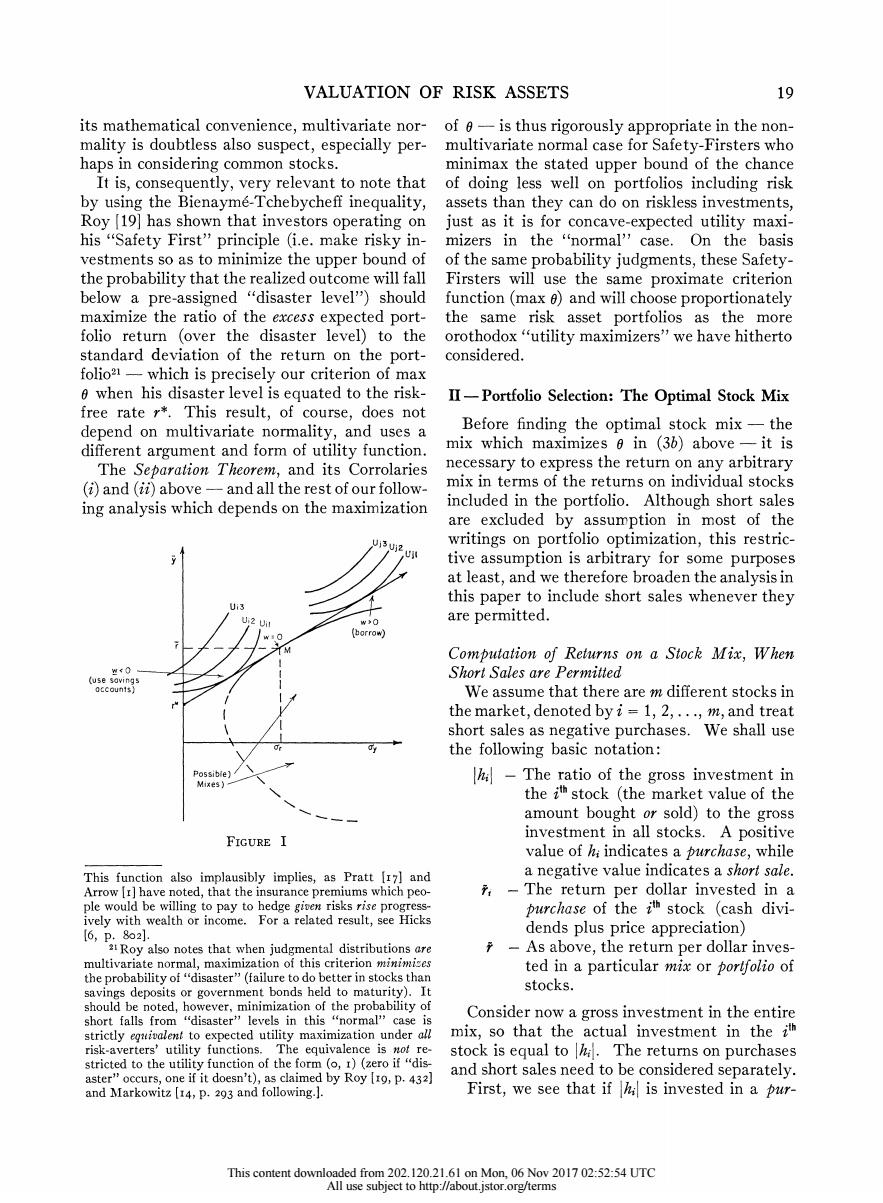
VALUATION OF RISK ASSETS 19 its mathematical convenience,multivariate nor-of-is thus rigorously appropriate in the non- mality is doubtless also suspect,especially per-multivariate normal case for Safety-Firsters who haps in considering common stocks. minimax the stated upper bound of the chance It is,consequently,very relevant to note that of doing less well on portfolios including risk by using the Bienayme-Tchebycheff inequality,assets than they can do on riskless investments, Roy [19]has shown that investors operating on just as it is for concave-expected utility maxi- his "Safety First"'principle (i.e.make risky in-mizers in the "normal''case.On the basis vestments so as to minimize the upper bound of of the same probability judgments,these Safety- the probability that the realized outcome will fall Firsters will use the same proximate criterion below a pre-assigned "disaster level")should function(max )and will choose proportionately maximize the ratio of the excess expected port-the same risk asset portfolios as the more folio return (over the disaster level)to the orothodox"utility maximizers"we have hitherto standard deviation of the return on the port-considered. folio2-which is precisely our criterion of max 0 when his disaster level is equated to the risk-II-Portfolio Selection:The Optimal Stock Mix free rate r*.This result,of course,does not depend on multivariate normality,and uses a Before finding the optimal stock mix-the different argument and form of utility function. mix which maximizes 0 in (36)above-it is The Separation Theorem,and its Corrolaries necessary to express the return on any arbitrary (i)and (ii)above-and all the rest of our follow- mix in terms of the returns on individual stocks ing analysis which depends on the maximization included in the portfolio.Although short sales are excluded by assumption in most of the writings on portfolio optimization,this restric- tive assumption is arbitrary for some purposes at least,and we therefore broaden the analysis in this paper to include short sales whenever they Ui3 Ui2 Uil w事O are permitted. (化orrow) Computation of Returns on a Stock Mix,When (use r0 Short Sales are Permitted We assume that there are m different stocks in the market,denoted by i=1,2,...,m,and treat short sales as negative purchases.We shall use the following basic notation: Possiblel -The ratio of the gross investment in the ith stock (the market value of the amount bought or sold)to the gross FIGURE I investment in all stocks.A positive value of hi indicates a purchase,while This function also implausibly implies,as Pratt [I7]and a negative value indicates a short sale. Arrow [r]have noted,that the insurance premiums which peo- -The return per dollar invested in a ple would be willing to pay to hedge gioen risks rise progress- purchase of the ith stock (cash divi- ively with wealth or income.For a related result,see Hicks I6,P.8o2l. dends plus price appreciation) a Roy also notes that when judgmental distributions are -As above,the return per dollar inves- multivariate normal,maximization of this criterion minimises ted in a particular mix or porlfolio of the probability of "disaster"(failure to do better in stocks than savings deposits or government bonds held to maturity).It stocks. should be noted,however,minimization of the probability of short falls from "disaster"levels in this "normal''case is Consider now a gross investment in the entire strictly eguivalent to expected utility maximization under all mix,so that the actual investment in the i risk-averters'utility functions.The equivalence is not re- stock is equal to The returns on purchases stricted to the utility function of the form (o,I)(zero if "dis- aster"occurs,one if it doesn't),as claimed by Roy [1o,p.432) and short sales need to be considered separately. and Markowitz [14,p.293 and following.]. First,we see that if is invested in a pur- This content downloaded from 202.120.21.61 on Mon,06 Nov 2017 02:52:54 UTC All use subject to http://about.jstor.org/terms
VALUATION OF RISK ASSETS 19 its mathematical convenience, multivariate nor- mality is doubtless also suspect, especially per- haps in considering common stocks. It is, consequently, very relevant to note that by using the Bienayme-Tchebycheff inequality, Roy [19] has shown that investors operating on his "Safety First" principle (i.e. make risky in- vestments so as to minimize the upper bound of the probability that the realized outcome will fall below a pre-assigned "disaster level") should maximize the ratio of the excess expected port- folio return (over the disaster level) to the standard deviation of the return on the port- folio2l - which is precisely our criterion of max 0 when his disaster level is equated to the risk- free rate r*. This result, of course, does not depend on multivariate normality, and uses a different argument and form of utility function. The Separation Theorem, and its Corrolaries (i) and (ii) above - and all the rest of our follow- ing analysis which depends on the maximization Uj3 Uj2 U1" Ui3 Ui2 U w>O o /27< (borrow) w < 0 (use savings accounts) / Possible) Mixes) FIGURE I of 0 - is thus rigorously appropriate in the non- multivariate normal case for Safety-Firsters who minimax the stated upper bound of the chance of doing less well on portfolios including risk assets than they can do on riskless investments, just as it is for concave-expected utility maxi- mizers in the "normal" case. On the basis of the same probability judgments, these Safety- Firsters will use the same proximate criterion function (max o) and will choose proportionately the same risk asset portfolios as the more orothodox "utility maximizers" we have hitherto considered. II -Portfolio Selection: The Optimal Stock Mix Before finding the optimal stock mix - the mix which maximizes 0 in (3b) above -it is necessary to express the return on any arbitrary mix in terms of the returns on individual stocks included in the portfolio. Although short sales are excluded by assumption in most of the writings on portfolio optimization, this restric- tive assumption is arbitrary for some purposes at least, and we therefore broaden the analysis in this paper to include short sales whenever they are permitted. Computation of Returns on a Stock Mix, When Short Sales are Permitted We assume that there are m different stocks in the market, denoted by i = 1, 2, .. ., m, and treat short sales as negative purchases. We shall use the following basic notation: -hil The ratio of the gross investment in the Pth stock (the market value of the amount bought or sold) to the gross investment in all stocks. A positive value of hi indicates a purchase, while a negative value indicates a short sale. - The return per dollar invested in a purchase of the Pth stock (cash divi- dends plus price appreciation) - As above, the return per dollar inves- ted in a particular mix or portfolio of stocks. Consider now a gross investment in the entire mix, so that the actual investment in the ith stock is equal to Ihil. The returns on purchases and short sales need to be considered separately. First, we see that if 1hil is invested in a pur- This function also implausibly implies, as Pratt |I 7] and Arrow [i] have noted, that the insurance premiums which peo- ple would be willing to pay to hedge given risks rise progress- ively with wealth or income. For a related result, see Hicks [6, p. 802]. 2'Roy also notes that when judgmental distributions are multivariate normal, maximization of this criterion minimizes the probability of "disaster" (failure to do better in stocks than savings deposits or government bonds held to maturity). It should be noted, however, minimization of the probability of short falls from "disaster" levels in this "normal" case is strictly eqiuivalent to expected utility maximization under all risk-averters' utility functions. The equivalence is not re- stricted to the utility function of the form (o, i) (zero if "dis- aster" occurs, one if it doesn't), as claimed by Roy [I9, P. 432] and Markowitz [I4, P. 293 and following.]. This content downloaded from 202.120.21.61 on Mon, 06 Nov 2017 02:52:54 UTC All use subject to http://about.jstor.org/terms
20 THE REVIEW OF ECONOMICS AND STATISTICS chase (0),the return will be simply hi.(5)=;[hr*)+r*] For reasons which will be clear immediately how- =r*十2h(行:一r*) ever,we write this in the form: because =I by the definition of. (4a)h:=h(f:-r*)+hlr* The expectation and variance of the return on Now suppose that is invested in a short any stock mix is consequently sale (h<o),this gross investment being equal (6a)平=Y*+2h:(r:-r*)=r*十hco to the price received for the stock.(The price (66)== received must be deposited in escrow,and in where;represents the variance when addition,an amount equal to margin require-i=j,and covariances whenij.The notation ments on the current price of the stock sold must has been further simplified in the right-hand be remitted or loaned to the actual owner of the expressions by defining: securities borrowed to effect the short sale.) (7)元:=7:一r*, In computing the return on a short sale,we and making appropriate substitutions in the know that the short seller must pay to the person who lends him the stock any dividends middle expressions.The quantity 6 defined in which accrue while the stock is sold short (and (3b)can thus be written: hence borrowed),and his capital gain (or loss) 元 (8) 日=户一* Eh is the negative of any price appreciation during ()12=()1e=(8h,h)12 this period.In addition,the short seller will Since k:may be either positive or negative, receive interest at the riskless rate r*on the equation (6a)shows that a portfolio with sales price placed in escrow,and he may or may 乎爻v*and hence with>o exists if there is not also receive interest at the same rate on his one or more stocks with:not exactly equal to cash remittance to the lender of the stock.To r*.We assume throughout the rest of the paper facilitate the formal analysis,we assume that that such a portfolio exists. both interest components are always received by the short seller,and that margin requirements are Determination of the Optimal Stock Porlfolio Iooo.In this case,the short seller's relurn per As shown in the proof of the Separation dollar of his gross investment will be (2r*-r),Theorem above,the optimal stock portfolio is and if he invests in the short sale (<o),the one which maximizes 0 as defined in equa- its contribution to his portfolio return will be:tion (8).We,of course,wish to maximize this (46)(ar*)=(-r*)+r*.value subject to the constraint Since the right-hand sides of (4a)and (4b)are (9):=I, identical,the total return per dollar invested in which follows from the definition of But any stock mix can be written as: we observe from equation(8)that 0 is a homog- eneous function of order zero in the h::the value 2In recent years,it has become increasingly common for the short seller to waive interest on his deposit with the lender of e is unchanged by any proportionale change in of the security-in market parlance,for the borrowers of all k.Our problem thus reduces to the simpler stock to obtain it"flat"-and when the demand for borrowing one of finding a vector of values yielding the stock is large relative to the supply available for this purpose, the borrower may pay a cash premium to the lender of the unconstrained maximum of 0 in equation (8), stock.See Sidney M.Robbins,[18,pp.58-591.It will be after which we may scale these initial solution noted that these practices reduce the expected return of short values to satisfy the constraint. sales without changing the variance.The formal procedures developed below permit the identification of the appropriate stocks for short sale assuming the expected return is (2r*-f) The Optimum Portfolio When Short Sales If these stocks were to be borrowed "flat"or a premium paid, are Permitted it would be simply necessary to iterate the solution after replacing (-r)in (4b)and (5)for these stocks with the value () We first examine the partial derivatives of(8) and if,in addition,a premium is paid,the term ( with respect to thek;and find: should be substituted (where p:2 o is the premium (if any) 88 per dollar of sales price of the stock to be paid to lender of the (Io) =(c)-1[e:-λ(h+2h)], stock).With equal lending and borrowing rates,changes in oh: margin requirements will not affect the calculations.(I am where, indebted to Prof.Schlaifer for suggesting the use of absolute values in analyzing short sales.) (II)λ=/g2=2hc/2:2hhi This content downloaded from 202.120.21.61 on Mon,06 Nov 2017 02:52:54 UTC All use subject to http://about.jstor.org/terms
20 THE REVIEW OF ECONOMICS AND STATISTICS chase (hi > 0), the return will be simply hiri. For reasons which will be clear immediately how- ever, we write this in the form: (4a) h?ir = h( i-r*) + IhiI r*. Now suppose that Ihi I is invested in a short sale (hi < o), this gross investment being equal to the price received for the stock. (The price received must be deposited in escrow, and in addition, an amount equal to margin require- ments on the current price of the stock sold must be remitted or loaned to the actual owner of the securities borrowed to effect the short sale.) In computing the return on a short sale, we know that the short seller must pay to the person who lends him the stock any dividends which accrue while the stock is sold short (and hence borrowed), and his capital gain (or loss) is the negative of any price appreciation during this period. In addition, the short seller will receive interest at the riskless rate r* on the sales price placed in escrow, and he may or may not also receive interest at the same rate on his cash remittance to the lender of the stock. To facilitate the formal analysis, we assume that both interest components are always received by the short seller, and that margin requirements are ioo%. In this case, the short seller's return per dollar of his gross investment will be (2r* -r), and if he invests Ih1iI in the short sale (hi< o), its contribution to his portfolio return will be: (4b) 1hi I (2r* - ri) = hi(fi - r*) + |hi I r*. Since the right-hand sides of (4a) and (4b) are identical, the total return per dollar invested in any stock mix can be written as: (5) r = i i - r*) + Ihilr*] =r* + 2ihi(fi - r*) because Ii Ihi I = i by the definition of Ihi I The expectation and variance of the return on any stock mix is consequently (6a) i = r* + ihi(,i - r*) = r* + lihizi, (6b) r = ijhihjrzij = 2ijhihz Iz where rii represents the variance ar,ij2 when i = j, and covariances when i # j. The notation has been further simplified in the right-hand expressions by defining: (7) xi = rj-r*J and making appropriate substitutions in the middle expressions. The quantity 0 defined in (3b) can thus be written: rr* xJZhi (8) 0 = r = (r) 1/2 (X)1/2 - ____ _1 /2 Since hi may be either positive or negative, equation (6a) shows that a portfolio with r> > r* and hence with 0 > o exists if there is one or more stocks with r- not exactly equal to r*. We assume throughout the rest of the paper that such a portfolio exists. Determination of the Optimal Stock Portfolio As shown in the proof of the Separation Theorem above, the optimal stock portfolio is the one which maximizes 0 as defined in equa- tion (8). We, of course, wish to maximize this value subject to the constraint (9) 2i hiI =I, which follows from the definition of Ihi 1. But we observe from equation (8) that 0 is a homog- eneous function of order zero in the hi: the value of 0 is unchanged by any proportionate change in all hi. Our problem thus reduces to the simpler one of finding a vector of values yielding the unconstrained maximum of 0 in equation (8), after which we may scale these initial solution values to satisfy the constraint. The Optimum Portfolio When Short Sales are Permitted We first examine the partial derivatives of (8) with respect to the hi and find: (IO) ah = (0x-l [xi-(i + 2;htjx) ], aoi where, (I I) X = /C1 _x2_v / v 22In recent years, it has become increasingly common for the short seller to waive interest on his deposit with the lender of the security - in market parlance, for the borrowers of stock to obtain it "flat"- and when the demand for borrowing stock is large relative to the supply available for this purpose, the borrower may pay a cash premium to the lender of the stock. See Sidney M. Robbins, [i8, pp. 58-59]. It will be noted that these practices reduce the expected return of short sales without changing the variance. The formal procedures developed below permit the identification of the appropriate stocks for short sale assuming the expected return is (2r* - ft). If these stocks were to be borrowed "flat" or a premium paid, it would be simply necessary to iterate the solution after replacing (j- r*) in (4b) and (5) for these stocks with the value (ii) - and if, in addition, a premium pi is paid, the term (ri + pi) should be substituted (where pi > o is the premium (if any) per dollar of sales price of the stock to be paid to lender of the stock). With equal lending and borrowing rates, changes in margin requirements will not affect the calculations. (I am indebted to Prof. Schlaifer for suggesting the use of absolute values in analyzing short sales.) This content downloaded from 202.120.21.61 on Mon, 06 Nov 2017 02:52:54 UTC All use subject to http://about.jstor.org/terms
VALUATION OF RISK ASSETS 21 The necessary and sufficient conditions on thethe sum of their absolute values.A comparison relative values of the h:for a stationary and the of equations (16)and (II)shows further that: unique (global)maximum23 are obtained by (18):=0=0/2; setting the derivatives in (Io)equal to zero, i.e.the sum of the absolute values of the which give the set of equations yields,as a byproduct,the value of the ratio of (12)8成十2=元,i=1,2,···,m; the expected excess rate of return on the optimal where we write portfolio to the variance of the return on this (I3)名=λh. best portfolio. It is also of interest to note that if we form the It will be noted the set of equations (12)- corresponding A-ratio of the expected excess which are identical to those Tobin derived by a return to its variance for each ith stock,we have different route24-are linear in the own-vari- at the optimum: ances,pooled covariances,and excess returns of the respective securities;and since the covariance (Ig)heo=(入/入)-2h,e/where matrix is positive definite and hence non- 入i=无/ci. singular,this system of equations has a unique The optimal fraction of each security in the best solution portfolio is equal to the ratio of its A;to that of the entire portfolio,less the ratio of its pooled (I4)80=2元; covariance with other securities to its own vari- where represents the ijth element of (ance.Consequently,if the investor were to act the inverse of the covariance matrix.Using on the assumption that all covariances were (13),(7),and (66),this solution may also be zero,he could pick his optimal portfolio mix written in terms of the primary variables of the very simply by determining the A:ratio of the problem in the form expected excess return元:=r:-r*of each (15)h0=(入)-12产f5-r*,alli. stock to its variance=,and setting each Moreover,since (13)implies h:=入/;for with no covariances,25zλt= (t6):z:|=λ2:lh:, A=2.With this simplifying assumption, the A:ratios of each stock suffice to determine Ao may readily be evaluated,after introducing the optimal mix by simple arithmetic;26 in the the constraint (9)as more general case with non-zero covariances,a (I7)2:z:0|=入2:h,0|=λ0 single set27 of linear equations must be solved in The optimal relative investments z:can conse- the usual way,but no (linear or non-linear) quently be scaled to the optimal proportions of programming is required and no more than one the stock portfolio h,by dividing each zr by point on the "efficient frontier"need ever be computed,given the assumptions under which 23It is clear from a comparison of equations (8)and (I), we are working. showing that sgn 0 sgn A,that only the vectors of values corresponding to>oare relevant to the maximization of 0. Moreover,since 6 as given in (8)and all its first partials shown The Optimum Portfolio When Short Sales in (Io)are continuous functions of the /it follows that when are not Permitted short sales are permitted,any maximum of 6 must be a station- The exclusion of short sales does not compli- ary value,and any stationary value is a maximum(rather than a minimum)when A>o because 0 is a convex function with a cate the above analysis if the investor is willing positive-definite quadratic torm in its denominator.For the to act on an assumption of no correlations same reason,any maximum of 6 is a unique(global)maximum. between the returns on different stocks.In this 2See Tobin,[21],equation (3.22),p.83.Tobin had,how- ever,formally required no short selling or borrowing,implying case,he finds his best portfolio of "long"holding that this set of equations is valid under these constraints [so by merely eliminating all securities whose A; long as there is a single riskless asset (pp.84-85);but the constraints were ignored in his derivation.We have shown 2s With no covariances,the set of equations (I2)reduces that this set of equations is valid when short sales are properly toλa=/ia=入i,and after summing over all i=I, included in the portfolio and borrowing is available in perfect 2...m,and using the constraint (9),we have immediately markets in unlimited amounts.The alternative set of equi- that|λo|=:|入,andλo>ofor max(instead of min) librium conditions required when short sales are ruled out is 24 Using a more restricted market setting,Hicks [6,p.8or] given immediately below.The complications introduced by has also reached an equivalent result when covariances are borrowing restrictions are examined in the final section of the zero (as he assumed throughout). paper. 27 See,however,footnote 22,above. This content downloaded from 202.120.21.61 on Mon,06 Nov 2017 02:52:54 UTC All use subject to http://about.jstor.org/terms
VALUATION OF RISK ASSETS 21 The necessary and sufficient conditions on the relative values of the hi for a stationary and the unique (global) maximum23 are obtained by setting the derivatives in (io) equal to zero, which give the set of equations (I2) Zitij + jZjaxij = i, i = I, 2, . . ,m; where we write (I3) zi = Xhi. It will be noted the set of equations (I 2)- which are identical to those Tobin derived by a different route24 -are linear in the own-vari- ances, pooled covariances, and excess returns of the respective securities; and since the covariance matrix xc is positive definite and hence non- singular, this system of equations has a unique solution (I4) zi? = 2jj where xii represents the i0th element of (x)-l the inverse of the covariance matrix. Using (I3), (7), and (6b), this solution may also be written in terms of the primary variables of the problem in the form (I5) hi? = (XO)-12jrii(j - r*), all i. Moreover, since (I3) implies (i6) 2zi I = X2h i, XO may readily be evaluated, after introducing the constraint (g) as (I 7) 2;i Izi? t i Ihi? I = ?o (~~) ~ = h0 The optimal relative investments zi? can conse- quently be scaled to the optimal proportions of the stock portfolio hi?, by dividing each zi? by the sum of their absolute values. A comparison of equations (i6) and (ii) shows further that: (i8) 2i -zi? I = ? = X?/a o2; i.e. the sum of the absolute values of the zi0 yields, as a byproduct, the value of the ratio of the expected excess rate of return on the optimal portfolio to the variance of the return on this best portfolio. It is also of interest to note that if we form the corresponding X-ratio of the expected excess return to its variance for each ith stock, we have at the optimum: (i9) hi? = (Xi/XO) - 2;j?xijiii where Xi = The optimal fraction of each security in the best portfolio is equal to the ratio of its Xi to that of the entire portfolio, less the ratio of its pooled covariance with other securities to its own vari- ance. Consequently, if the investor were to act on the assumption that all covariances were zero, he could pick his optimal portfolio mix very simply by determining the Xi ratio of the expected excess return xi = i- r* of each stock to its variance xij = rii, and setting each hi= Xi/2Xi; for with no covariances,25 2Ai = XO = 0/1ae2. With this simplifying assumption, the Xi ratios of each stock suffice to determine the optimal mix by simple arithmetic;26 in the more general case with non-zero covariances, a single set27 of linear equations must be solved in the usual way, but no (linear or non-linear) programming is required and no more than one point on the "efficient frontier" need ever be computed, given the assumptions under which we are working. The Optimum Portfolio When Short Sales are not Permitted The exclusion of short sales does not compli- cate the above analysis if the investor is willing to act on an assumption of no correlations between the returns on different stocks. In this case, he finds his best portfolio of "long" holding by merely eliminating all securities whose Xi- 231t is clear from a comparison of equations (8) and (ii), showing that sgn 0 = sgn X, that only the vectors of hi values corresponding to X > o are relevant to the maximization of 0. Moreover, since 0 as given in (8) and all its first partials shown in (io) are continuous functions of the hi, it follows that when short sales are permitted, any maximum of 0 must be a station- ary value, and any stationary value is a maximum (rather than a minimum) when X > o because 0 is a convex function with a positive-definite quadratic torm in its denominator. For the same reason, any maximum of 0 is a unique (global) maximum. 24See Tobin, [2I], equation (3.22), p. 83. Tobin had, how- ever, formally required no short selling or borrowing, implying that this set of equations is valid under these constraints [so long as there is a single riskless asset (pp. 84-85)]; but the constraints were ignored in his derivation. We have shown that this set of equations is valid when short sales are properly included in the portfolio and borrowing is available in perfect markets in unlimited amounts. The alternative set of equi- librium conditions required when short sales are ruled out is given immediately below. The complications introduced by borrowing restrictions are examined in the final section of the paper. 25 With no covariances, the set of equations (I2) reduceS to Xhs = = Xi, and after summing over all i =I, 2 ... m, and using the constraint (9), we have immediately that I X 0 = Ii I Xi 1, and X > o for max 0 (instead of min 0). 26 Using a more restricted market setting, Hicks [6, p. 8oi] has also reached an equivalent result when covariances are zero (as he assumed throughout). 27 See, however, footnote 22, above. This content downloaded from 202.120.21.61 on Mon, 06 Nov 2017 02:52:54 UTC All use subject to http://about.jstor.org/terms