430 The Journal of Finance If the proportion a of the individual's wealth is placed in plan A and the remainder(1-a)in B,the expected rate of return of the combination will lie between the expected returns of the two plans: ERe=aERa十(1一a)ERb The predicted standard deviation of return of the combination is: 0Re=Va2ora2十(1一a)20rb2+2raba(1一a)Ragb Note that this relationship includes rab,the correlation coefficient between the predicted rates of return of the two investment plans.A value of +1 would indicate an investor's belief that there is a precise positive relation- ship between the outcomes of the two investments.A zero value would indicate a belief that the outcomes of the two investments are completely independent and-1 that the investor feels that there is a precise inverse relationship between them.In the usual case rab will have a value between 0 and +1. Figure 3 shows the possible values of Ere and oRe obtainable with different combinations of A and B under two different assumptions about oRb 0R3 Z pRo 如 FIGURE 3 This content downloaded from 202.120.21.61 on Mon,06 Nov 2017 02:56:13 UTC All use subject to http://about.istor.org/terms
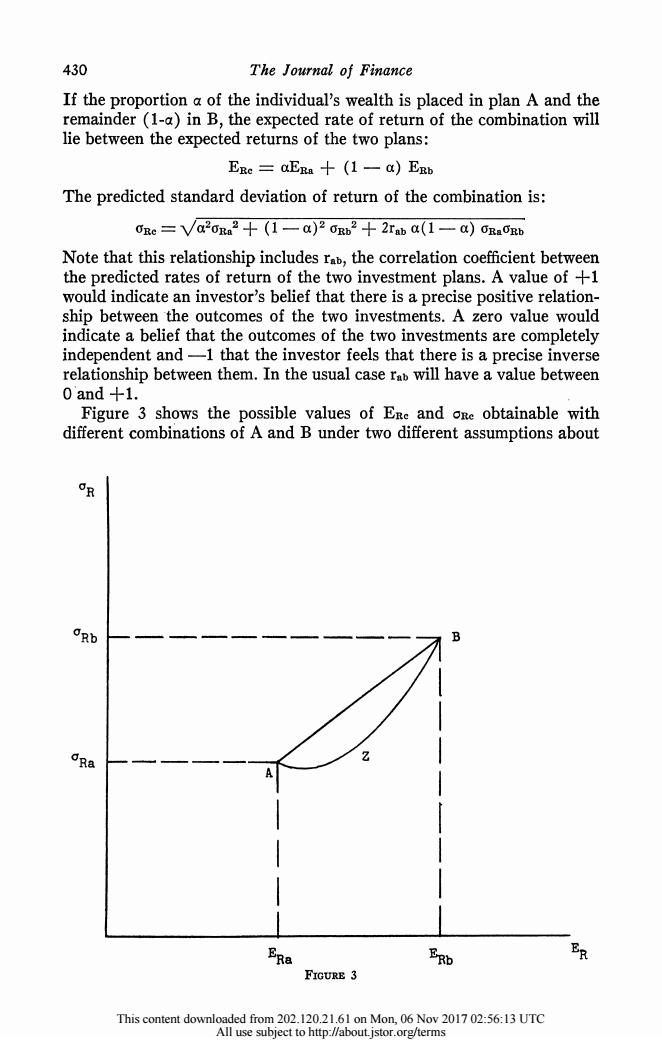
430 The Journal of Finance If the proportion a of the individual's wealth is placed in plan A and the remainder (1-a) in B, the expected rate of return of the combination will lie between the expected returns of the two plans: ER= aERa + (1 a) ERb The predicted standard deviation of return of the combination is: RC Va2Ra 2 + (1 a)2 Rb2 + 2rab a(1 - a) CRaORb Note that this relationship includes rab, the correlation coefficient between the predicted rates of return of the two investment plans. A value of +1 would indicate an investor's belief that there is a precise positive relation- ship between 'the outcomes of the two investments. A zero value would indicate a belief that the outcomes of the two investments are completely independent and -1 that the investor feels that there is a precise inverse relationship between them. In the usual case rab will have a value between o and +1. Figure 3 shows the possible values of ERc and ORC obtainable with different combinations of A and B under two different assumptions about OR aRb -B CRa- I I l I I I ERa ERb ER FIGURE 3 This content downloaded from 202.120.21.61 on Mon, 06 Nov 2017 02:56:13 UTC All use subject to http://about.jstor.org/terms
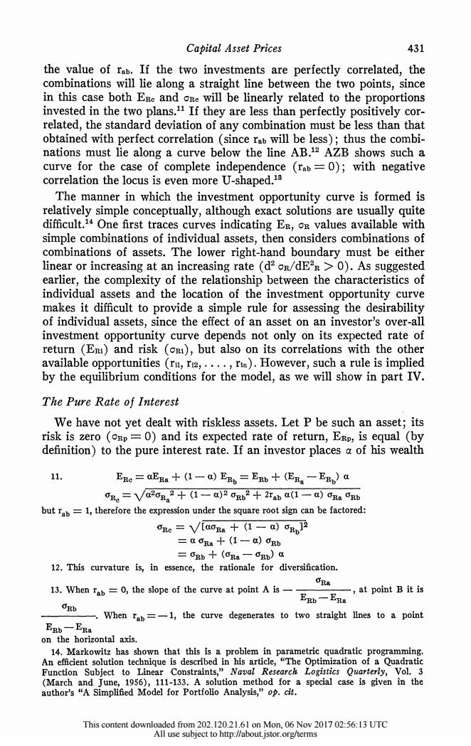
Capital Asset Prices 431 the value of rab.If the two investments are perfectly correlated,the combinations will lie along a straight line between the two points,since in this case both ERe and one will be linearly related to the proportions invested in the two plans.If they are less than perfectly positively cor- related,the standard deviation of any combination must be less than that obtained with perfect correlation (since rab will be less);thus the combi- nations must lie along a curve below the line AB.12 AZB shows such a curve for the case of complete independence (rab=0);with negative correlation the locus is even more U-shaped.18 The manner in which the investment opportunity curve is formed is relatively simple conceptually,although exact solutions are usually quite difficult.14 One first traces curves indicating Er,on values available with simple combinations of individual assets,then considers combinations of combinations of assets.The lower right-hand boundary must be either linear or increasing at an increasing rate (d2 on/dE2R>0).As suggested earlier,the complexity of the relationship between the characteristics of individual assets and the location of the investment opportunity curve makes it difficult to provide a simple rule for assessing the desirability of individual assets,since the effect of an asset on an investor's over-all investment opportunity curve depends not only on its expected rate of return (ER)and risk (cR),but also on its correlations with the other available opportunities (ru,r2,....,r).However,such a rule is implied by the equilibrium conditions for the model,as we will show in part IV. The Pure Rate of Interest We have not yet dealt with riskless assets.Let P be such an asset;its risk is zero (cEp=0)and its expected rate of return,Erp,is equal (by definition)to the pure interest rate.If an investor places a of his wealth 11. ERe=ERa十(I一a)ERb=ERb+(ERa一ER,)a ORe=Va20B 2+(1-a)2 ORb2+2Tab a(1-a)GRa Ogb but rab=1,therefore the expression under the square root sign can be factored: oRe=V儿a0Ra+((1-a)r, =a ORa +(1-a)ORb =Rb+(CRa一ORb)a 12.This curvature is,in essence,the rationale for diversification. ORa 13.When rab =0,the slope of the curve at point A is- -at point B it is ERb一ER ORb -When rab=-1,the curve degenerates to two straight lines to a point ERb一ER on the horizontal axis. 14.Markowitz has shown that this is a problem in parametric quadratic programming. An efficient solution technique is described in his article,"The Optimization of a Quadratic Function Subject to Linear Constraints,"Naval Research Logistics Quarterly,Vol.3 (March and June,1956),111-133.A solution method for a special case is given in the author's "A Simplified Model for Portfolio Analysis,"op.cit. This content downloaded from 202.120.21.61 on Mon,06 Nov 2017 02:56:13 UTC All use subject to http://about.istor.org/terms
Capital Asset Prices 431 the value of rab. If the two investments are perfectly correlated, the combinations will lie along a straight line between the two points, since in this case both ERC and oRc will be linearly related to the proportions invested in the two plans.11 If they are less than perfectly positively cor- related, the standard deviation of any combination must be less than that obtained with perfect correlation (since rab will be less); thus the combi- nations must lie along a curve below the line AB."2 AZB shows such a curve for the case of complete independence (rab - 0); with negative correlation the locus is even more U-shaped.13 The manner in which the investment opportunity curve is formed is relatively simple conceptually, although exact solutions are usually quite difficult.14 One first traces curves indicating ER, OR values available with simple combinations of individual assets, then considers combinations of combinations of assets. The lower right-hand boundary must be either linear or increasing at an increasing rate (d2 CR/dE2R> 0). As suggested earlier, the complexity of the relationship between the characteristics of individual assets and the location of the investment opportunity curve makes it difficult to provide a simple rule for assessing the desirability of individual assets, since the effect of an asset on an investor's over-all investment opportunity curve depends not only on its expected rate of return (ERI) and risk (CR1), but also on its correlations with the other available opportunities (rii, rI2 ...., rin). However, such a rule is implied by the equilibrium conditions for the model, as we will show in part IV. The Pure Rate of Interest We have not yet dealt with riskless assets. Let P be such an asset; its risk is zero (oRp = 0) and its expected rate of return, ERR, is equal (by definition) to the pure interest rate. If an investor places a of his wealth 11. ERC = aERa + (1 -a) ERb = ERb + (ERa ERb) ORC = V/a2Ra2 + (1- a)2 cvRb2 + 2rab a(1 - a) rRa aRb butab 1, therefore the expression under the square root sign can be factored: YRc = \/[aaRa + (1 GO) cRb]2 - a YRa + (1 - a) aRb - 0Rb + (OYRa - YRb) a 12. This curvature is, in essence, the rationale for diversification. 13. When rab = 0, the slope of the curve at point A is - , at point B it is ERb - ERa YRb . When rab =-1, the curve degenerates to two straight lines to a point ERb- ERa on the horizontal axis. 14. Markowitz has shown that this is a problem in parametric quadratic programming. An efficient solution technique is described in his article, "The Optimization of a Quadratic Function Subject to Linear Constraints," Naval Research Logistics Quarterly, Vol. 3 (March and June, 1956), 111-133. A solution method for a special case is given in the author's "A Simplified Model for Portfolio Analysis," op. cit. This content downloaded from 202.120.21.61 on Mon, 06 Nov 2017 02:56:13 UTC All use subject to http://about.jstor.org/terms