Site 31.55 4.30 15 602.413e-05*** Residuals 22 Signif.c0des:0J**’0.0013**’0.01’*’0.05’.’0.1’’1 There is,therefore,strong evidence against the null hypothesis of no differences in mean vectors across sites. 4.2 Two-Way MANOVA:Plastic Film Data For a slightly more complex example,we use textbook data from Johnson and Wichern (1992:266)on an experiment conducted to determine the optimum conditions for extruding plastic film.Three responses(tear resistance,film gloss,and opacity)were measured in relation to two factors:rate of extrusion (Low/High) and amount of an additive (Low/High).Again,the data are in the heplots package: Plastic tear gloss opacity rate additive 1 6.59.5 4.4 Low LoW 6.2 9.9 6.4 Low Low 3 5.8 9.6 3.0L0w LoW 4 6.5 9.6 4.1 Low LOW 6.5 9.2 0.8 Low LoW 6 6.9 9.1 5.7 Low High 7 7.2 10.0 2.0 Low High 6.9 9.9 3.9 Low Hig融 9 6.1 9.5 1.9 Low High 10 6.3 9.4 5.7 Low Hig助 11 6.7 9.1 2.8 High LOW 12 6.6 9.3 4.1 High LOW 13 7.2 8.3 3.8 High Low 14 7.1 8.4 1.6 High LOW 15 6.8 8.5 3.4 High LOw 16 7.1 9.2 8.4 High High 17 7.0 8.8 5.2 High High 18 7.2 9.7 6.9 High High 19 7.5 10.1 2.7 High High 20 7.6 9.2 1.9 High High We fit the two-way MANOVA model and display the Anova results,using Roy's maximum root test. Both main effects are significant,but their interaction is not: plastic.mod <-lm(cbind(tear,gloss,opacity)~rate*additive,data=Plastic) Anova(plastic.mod,test.statistic="Roy") Type II MANOVA Tests:Roy test statistic Df test stat approx F num Df den Df Pr(>F) rate 1 1.61887.5543 3 140.003034** additive 1 0.9119 4.2556 3 140.024745* rate:additive 1 0.28681.3385 3 140.301782 Sig题if.c0des:0’**?0.001’*30.01’*’0.05).’0.1’)1 Again,we get the same tests from anova,this time because the data are balanced (so that sequential and Type-II tests coincide): 6
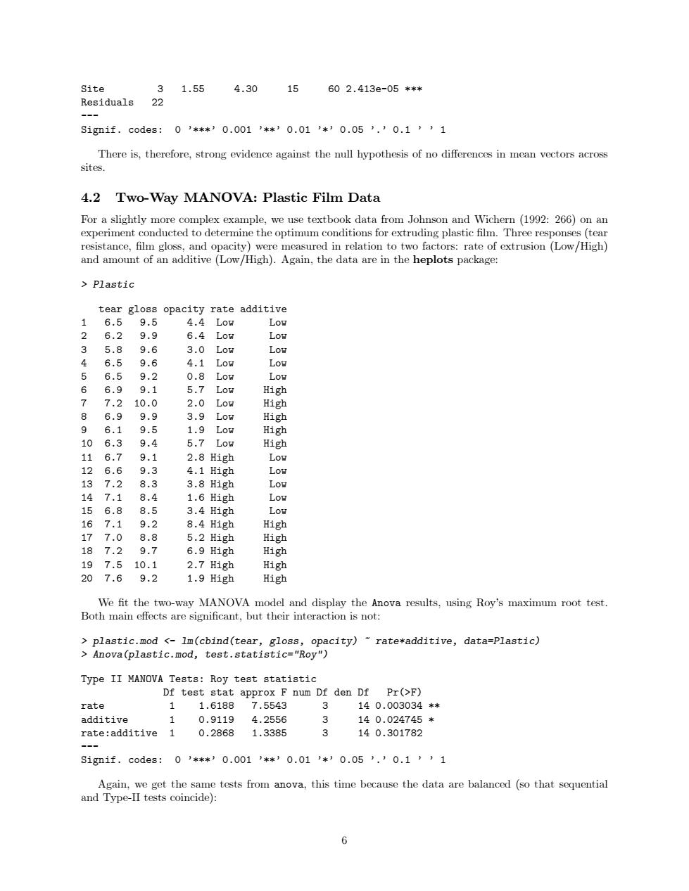
Site 3 1.55 4.30 15 60 2.413e-05 *** Residuals 22 --- Signif. codes: 0 ’***’ 0.001 ’**’ 0.01 ’*’ 0.05 ’.’ 0.1 ’ ’ 1 There is, therefore, strong evidence against the null hypothesis of no differences in mean vectors across sites. 4.2 Two-Way MANOVA: Plastic Film Data For a slightly more complex example, we use textbook data from Johnson and Wichern (1992: 266) on an experiment conducted to determine the optimum conditions for extruding plastic film. Three responses (tear resistance, film gloss, and opacity) were measured in relation to two factors: rate of extrusion (Low/High) and amount of an additive (Low/High). Again, the data are in the heplots package: > Plastic tear gloss opacity rate additive 1 6.5 9.5 4.4 Low Low 2 6.2 9.9 6.4 Low Low 3 5.8 9.6 3.0 Low Low 4 6.5 9.6 4.1 Low Low 5 6.5 9.2 0.8 Low Low 6 6.9 9.1 5.7 Low High 7 7.2 10.0 2.0 Low High 8 6.9 9.9 3.9 Low High 9 6.1 9.5 1.9 Low High 10 6.3 9.4 5.7 Low High 11 6.7 9.1 2.8 High Low 12 6.6 9.3 4.1 High Low 13 7.2 8.3 3.8 High Low 14 7.1 8.4 1.6 High Low 15 6.8 8.5 3.4 High Low 16 7.1 9.2 8.4 High High 17 7.0 8.8 5.2 High High 18 7.2 9.7 6.9 High High 19 7.5 10.1 2.7 High High 20 7.6 9.2 1.9 High High We fit the two-way MANOVA model and display the Anova results, using Roy’s maximum root test. Both main effects are significant, but their interaction is not: > plastic.mod <- lm(cbind(tear, gloss, opacity) ~ rate*additive, data=Plastic) > Anova(plastic.mod, test.statistic="Roy") Type II MANOVA Tests: Roy test statistic Df test stat approx F num Df den Df Pr(>F) rate 1 1.6188 7.5543 3 14 0.003034 ** additive 1 0.9119 4.2556 3 14 0.024745 * rate:additive 1 0.2868 1.3385 3 14 0.301782 --- Signif. codes: 0 ’***’ 0.001 ’**’ 0.01 ’*’ 0.05 ’.’ 0.1 ’ ’ 1 Again, we get the same tests from anova, this time because the data are balanced (so that sequential and Type-II tests coincide): 6
anova(plastic.mod,test="Roy") Analysis of Variance Table Df Roy approx F num Df den Df Pr(>F) (Intercept) 11275.2 5950.9 心 14<2.2e-16*** rate 1.6 7.6 3 140.003034* additive 1 0.9 4.3 3 14 0.024745* rate:additive 1 0.3 1.3 3 140.301782 Residuals 16 S1gnif.c0de8:0’***)0.001’**30.013*’0.05’.10.13’1 4.3 Multivariate Multiple Regression and MANCOVA:Rohwer Data In multivariate multiple regression,the X matrix contains quantitative predictors,while in multivariate analysis of covariance(MANCOVA),there is a mixture of factors and quantitative predictors(covariates).To illustrate,we use data from a study by Rohwer(given in Timm,1975:Ex.4.3,4.7,and 4.23)on kindergarten children,designed to determine how well a set of paired-associate (PA)tasks predicted performance on the Peabody Picture Vocabulary test (PPVT),a student achievement test (SAT),and the Raven Progressive matrices test (Raven).The PA tasks varied in how the stimuli were presented,and are called named (n), still (s),named still (ns),named action (na),and sentence still(ss).Two groups were tested:a group of n =37 children from a low socioeconomic status(SES)school,and a group of n 32 high SES children from an upper-class,white residential school.The data are in the data frame Rohwer in the heplots package: Rohwer group SES SAT PPVT Raven n s ns na ss 1L049 48 81261216 2 1L047 76 13514143027 3 1L011 40 13010211616 68 2Hi98 74 1526142517 69 2H15078 19510182726 Initially (and optimistically),we fit the MANCOVA model that allows different means for the two SES groups on the responses,but constrains the slopes for the PA covariates to be equal. rohwer.mod <-1m(cbind(SAT,PPVT,Raven)-SES n +s ns na ss, data=Rohwer) Anova(rohwer.mod) Type II MANOVA Tests:Pillai test statistic Df test stat approx F num Df den Df Pr(>F) SES 1 0.378512.1818 602.507e-06*** ◇ 1 0.0403 0.8400 3 60 0.477330 8 0.0927 2.0437 600.117307 ns 1 0.1928 4.7779 600.004729** na 1 0.2313 6.0194 600.001181** 88 1 0.0499 1.0504 3 600.376988 S1gmif.codes:0’**’0.001’*’0.01’*’0.05’.’0.1’’1 This multivariate linear model is of interest because,although the multivariate tests for two of the covariates (ns and na)are highly significant.univariate multiple regression tests for the separate responses [from summary(rohwer.mod)]are relatively weak.We can test the 5 df hypothesis that all covariates have null effects for all responses as a linear hypothesis (suppressing display of the error and hypothesis SSP matrices)
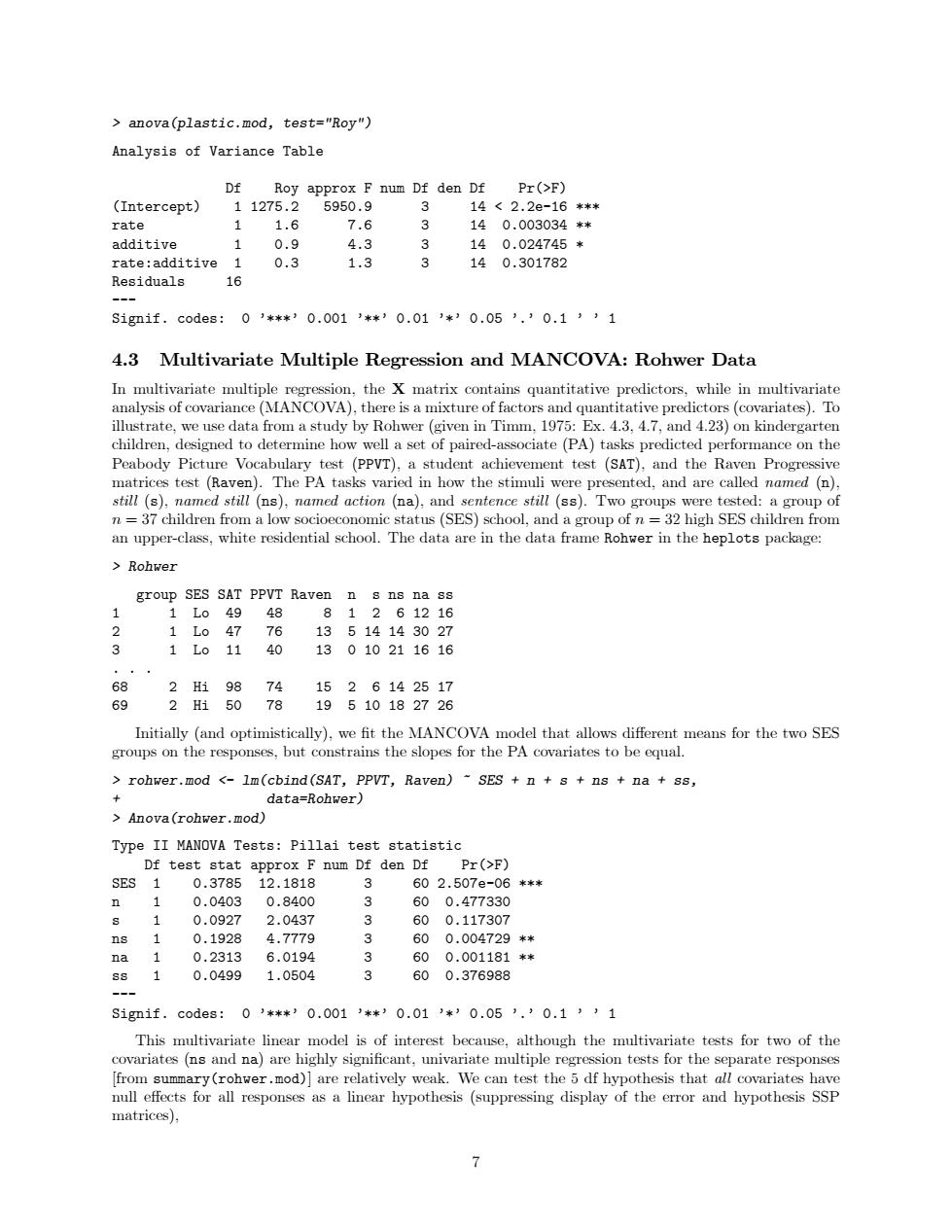
> anova(plastic.mod, test="Roy") Analysis of Variance Table Df Roy approx F num Df den Df Pr(>F) (Intercept) 1 1275.2 5950.9 3 14 < 2.2e-16 *** rate 1 1.6 7.6 3 14 0.003034 ** additive 1 0.9 4.3 3 14 0.024745 * rate:additive 1 0.3 1.3 3 14 0.301782 Residuals 16 --- Signif. codes: 0 ’***’ 0.001 ’**’ 0.01 ’*’ 0.05 ’.’ 0.1 ’ ’ 1 4.3 Multivariate Multiple Regression and MANCOVA: Rohwer Data In multivariate multiple regression, the X matrix contains quantitative predictors, while in multivariate analysis of covariance (MANCOVA), there is a mixture of factors and quantitative predictors (covariates). To illustrate, we use data from a study by Rohwer (given in Timm, 1975: Ex. 4.3, 4.7, and 4.23) on kindergarten children, designed to determine how well a set of paired-associate (PA) tasks predicted performance on the Peabody Picture Vocabulary test (PPVT), a student achievement test (SAT), and the Raven Progressive matrices test (Raven). The PA tasks varied in how the stimuli were presented, and are called named (n), still (s), named still (ns), named action (na), and sentence still (ss). Two groups were tested: a group of n = 37 children from a low socioeconomic status (SES) school, and a group of n = 32 high SES children from an upper-class, white residential school. The data are in the data frame Rohwer in the heplots package: > Rohwer group SES SAT PPVT Raven n s ns na ss 1 1 Lo 49 48 8 1 2 6 12 16 2 1 Lo 47 76 13 5 14 14 30 27 3 1 Lo 11 40 13 0 10 21 16 16 ... 68 2 Hi 98 74 15 2 6 14 25 17 69 2 Hi 50 78 19 5 10 18 27 26 Initially (and optimistically), we fit the MANCOVA model that allows different means for the two SES groups on the responses, but constrains the slopes for the PA covariates to be equal. > rohwer.mod <- lm(cbind(SAT, PPVT, Raven) ~ SES + n + s + ns + na + ss, + data=Rohwer) > Anova(rohwer.mod) Type II MANOVA Tests: Pillai test statistic Df test stat approx F num Df den Df Pr(>F) SES 1 0.3785 12.1818 3 60 2.507e-06 *** n 1 0.0403 0.8400 3 60 0.477330 s 1 0.0927 2.0437 3 60 0.117307 ns 1 0.1928 4.7779 3 60 0.004729 ** na 1 0.2313 6.0194 3 60 0.001181 ** ss 1 0.0499 1.0504 3 60 0.376988 --- Signif. codes: 0 ’***’ 0.001 ’**’ 0.01 ’*’ 0.05 ’.’ 0.1 ’ ’ 1 This multivariate linear model is of interest because, although the multivariate tests for two of the covariates (ns and na) are highly significant, univariate multiple regression tests for the separate responses [from summary(rohwer.mod)] are relatively weak. We can test the 5 df hypothesis that all covariates have null effects for all responses as a linear hypothesis (suppressing display of the error and hypothesis SSP matrices), 7
Regr <-linear.hypothesis(rohwer.mod,diag(7)[3:7,] print(Regr,digits=5,SSP=FALSE) Multivariate Tests: Df test stat approx F num Df den Df Pr(>F) Pillai 5.00 0.6658 3.536915.00186.002.309e-05*** Wilks 5.00 0.4418 3.811815.00166.038.275e-06*** Hotelling-Lawley 5.00 1.0309 4.032115.00176.002.787e-06*** Roy 5.00 0.7574 9.39245.0062,001,062e-06*** -- S1gif.codes:0’**’0.001’*’0.01’*’0.05’.’0.1’’1 As explained,in the MANCOVA model rohwer.mod we have assumed homogeneity of slopes for the predictors,and the test of SES relies on this assumption.We can test this as follows,adding interactions of SES with each of the covariates: rohwer.mod2 <-1m(cbind(SAT,PPVT,Raven)-SES (n +s +ns na ss), data=Rohwer) Anova(rohwer.mod2) Type II MANOVA Tests:Pillai test statistic Df test stat approx F num Df den Df Pr(>F) SES 1 0.391211,7822 3 55 4,55e-06**米 n 0.0790 1.5727 550.2063751 8 0.1252 2.6248 3 550.0595192 ns 1 0.2541 6.2461 3 550.0009995*** na 0.3066 8.1077 0 550.0001459*** 88 1 0.0602 1.1738 3 550.3281285 SES:n 1 0.0723 1.4290 550.2441738 SES:s 0.0994 2.0240 3 550.1211729 SES:ns 1 0.1176 2.4425 550.0738258 SES:na 0.1480 3.1850 550.0308108* SES:ss 0.0573 1.1150 550.3509357 S1g即if.codes:0’**’0.001’*’0.01’*)0.05’.’0.1’’1 It appears from the above that there is only weak evidence of unequal slopes from the separate SES: terms.The evidence for heterogeneity is stronger,however,when these terms are tested collectively using the linear.hypothesis function: >(coefs <-rownames(coef(rohwer.mod2))) [1]"(Intercept)""SESLo" "n" "ns" [6]"na" "88" "SESLo:n" "SESLO:S" "SESLo:ns" [11]"SESLo:na" "SESLo:ss" print(linear.hypothesis(rohwer.mod2,coefs [grep(":"coefs)]),SSP=FALSE) Multivariate Tests: Df test stat approx F num Df den Df Pr(>F) Pillai 5.00000.4179381.84522615.0000171.00000.0320861* Wilks 5.00000.6235821.89361315.0000152.23220.0276949* Hotelling-Lawley 5.00000.5386511.927175 15.0000161.00000.0239619* Roy 5.00000.3846494.384997 5.000057.00000.0019053** Signif.codes: 03***30.0013**30.013*)0.053.30.1331 8
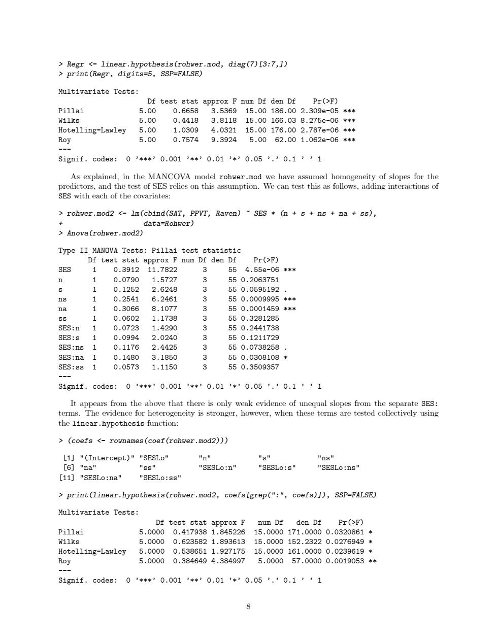
> Regr <- linear.hypothesis(rohwer.mod, diag(7)[3:7,]) > print(Regr, digits=5, SSP=FALSE) Multivariate Tests: Df test stat approx F num Df den Df Pr(>F) Pillai 5.00 0.6658 3.5369 15.00 186.00 2.309e-05 *** Wilks 5.00 0.4418 3.8118 15.00 166.03 8.275e-06 *** Hotelling-Lawley 5.00 1.0309 4.0321 15.00 176.00 2.787e-06 *** Roy 5.00 0.7574 9.3924 5.00 62.00 1.062e-06 *** --- Signif. codes: 0 ’***’ 0.001 ’**’ 0.01 ’*’ 0.05 ’.’ 0.1 ’ ’ 1 As explained, in the MANCOVA model rohwer.mod we have assumed homogeneity of slopes for the predictors, and the test of SES relies on this assumption. We can test this as follows, adding interactions of SES with each of the covariates: > rohwer.mod2 <- lm(cbind(SAT, PPVT, Raven) ~ SES * (n + s + ns + na + ss), + data=Rohwer) > Anova(rohwer.mod2) Type II MANOVA Tests: Pillai test statistic Df test stat approx F num Df den Df Pr(>F) SES 1 0.3912 11.7822 3 55 4.55e-06 *** n 1 0.0790 1.5727 3 55 0.2063751 s 1 0.1252 2.6248 3 55 0.0595192 . ns 1 0.2541 6.2461 3 55 0.0009995 *** na 1 0.3066 8.1077 3 55 0.0001459 *** ss 1 0.0602 1.1738 3 55 0.3281285 SES:n 1 0.0723 1.4290 3 55 0.2441738 SES:s 1 0.0994 2.0240 3 55 0.1211729 SES:ns 1 0.1176 2.4425 3 55 0.0738258 . SES:na 1 0.1480 3.1850 3 55 0.0308108 * SES:ss 1 0.0573 1.1150 3 55 0.3509357 --- Signif. codes: 0 ’***’ 0.001 ’**’ 0.01 ’*’ 0.05 ’.’ 0.1 ’ ’ 1 It appears from the above that there is only weak evidence of unequal slopes from the separate SES: terms. The evidence for heterogeneity is stronger, however, when these terms are tested collectively using the linear.hypothesis function: > (coefs <- rownames(coef(rohwer.mod2))) [1] "(Intercept)" "SESLo" "n" "s" "ns" [6] "na" "ss" "SESLo:n" "SESLo:s" "SESLo:ns" [11] "SESLo:na" "SESLo:ss" > print(linear.hypothesis(rohwer.mod2, coefs[grep(":", coefs)]), SSP=FALSE) Multivariate Tests: Df test stat approx F num Df den Df Pr(>F) Pillai 5.0000 0.417938 1.845226 15.0000 171.0000 0.0320861 * Wilks 5.0000 0.623582 1.893613 15.0000 152.2322 0.0276949 * Hotelling-Lawley 5.0000 0.538651 1.927175 15.0000 161.0000 0.0239619 * Roy 5.0000 0.384649 4.384997 5.0000 57.0000 0.0019053 ** --- Signif. codes: 0 ’***’ 0.001 ’**’ 0.01 ’*’ 0.05 ’.’ 0.1 ’ ’ 1 8