PART II JUSTIFICATIONS, COMPOSITE BEAMS, AND THICK PLATES We regroup in Part III elements that are less utilized than those in the previous parts.Nevertheless they are of fundamental interest for a better understanding of the principles for calculation of composite components.In the first two chapters, we focused on anisotropic properties and fracture strength of orthotropic materials, and then more particularly on transversely isotropic ones.The following two chapters allow us to consider that composite components in the form of beams can be "homogenized."This means that their study is analogous to the study of homogeneous beams that are common in the literature.Finally,the last chapter in this part describes with a similar procedure the behavior of thick composite plates subject to transverse loadings. 2003 by CRC Press LLC
PART III JUSTIFICATIONS, COMPOSITE BEAMS, AND THICK PLATES We regroup in Part III elements that are less utilized than those in the previous parts. Nevertheless they are of fundamental interest for a better understanding of the principles for calculation of composite components. In the first two chapters, we focused on anisotropic properties and fracture strength of orthotropic materials, and then more particularly on transversely isotropic ones. The following two chapters allow us to consider that composite components in the form of beams can be “homogenized.” This means that their study is analogous to the study of homogeneous beams that are common in the literature. Finally, the last chapter in this part describes with a similar procedure the behavior of thick composite plates subject to transverse loadings. TX846_Frame_C13 Page 257 Monday, November 18, 2002 12:29 PM © 2003 by CRC Press LLC
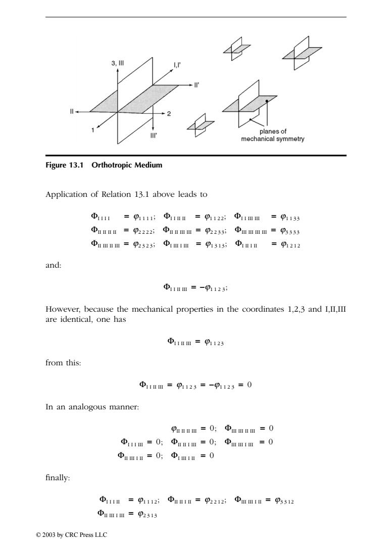
13 ELASTIC COEFFICIENTS The definition of a linear elastic anisotropic medium was given in Chapter 9.We have also given,without justification,the behavior relations characterizing the particular case of orthotropic materials.Now we propose to examine more closely the elastic constants which appear in stress-strain relations for these materials.In the case of transversely isotropic materials,we will study also the manner in which the constants evolve. 13.1 ELASTIC COEFFICIENTS IN AN ORTHOTROPIC MATERIAL Recall:Consider the relation for elastic behavior written in Paragraph 9.1.1 in the form: Emn Omnpqx Opq Recall that the components of a tensor expressed in the coordinate system 1,2,3 are written as du in a coordinate system I,II,II using the relation: UKL=cosT coSf cosk cos?Pmnpa (13.1) in which: cos”=cos(m,7 By definition,'for mechanical behavior,an orthotropic medium has at any point two orthogonal planes of symmetry.Consider here two coordinate systems 1,2,3 and I,II,III,constructed on these planes and their intersection.One plane can be obtained from the other by a 1800 rotation about the 3 axis as shown in Figure 13.1.One can deduce [-10 [cos"] 0-1 0 001 TSee Section 9.2. 2003 by CRC Press LLC
13 ELASTIC COEFFICIENTS The definition of a linear elastic anisotropic medium was given in Chapter 9. We have also given, without justification, the behavior relations characterizing the particular case of orthotropic materials. Now we propose to examine more closely the elastic constants which appear in stress–strain relations for these materials. In the case of transversely isotropic materials, we will study also the manner in which the constants evolve. 13.1 ELASTIC COEFFICIENTS IN AN ORTHOTROPIC MATERIAL Recall: Consider the relation for elastic behavior written in Paragraph 9.1.1 in the form: Recall that the components jmnpq of a tensor expressed in the coordinate system 1,2,3 are written as FIJKL in a coordinate system I,II,II using the relation: (13.1) in which: By definition,1 for mechanical behavior, an orthotropic medium has at any point two orthogonal planes of symmetry. Consider here two coordinate systems 1,2,3 and I,II,III, constructed on these planes and their intersection. One plane can be obtained from the other by a 180∞ rotation about the 3 axis as shown in Figure 13.1. One can deduce 1 See Section 9.2. emn = jmnpq ¥ spq FIJKL cosI m cosJ n cosK p cosL q = jmnpq cosI m = cos( ) m, I cosI m [ ] –1 0 0 0 1– 0 0 01 = TX846_Frame_C13 Page 259 Monday, November 18, 2002 12:29 PM © 2003 by CRC Press LLC
3,川 planes of mechanical symmetry Figure 13.1 Orthotropic Medium Application of Relation 13.1 above leads to Φ111=p1111;Φ1mm=p1122;④11mm=p1133 ①mmmm=p2222;Φunmm=p2233中mmmm=p3333 Φummm=p2323;④1m1m=p1313;④1n=p1212 and: Φ11Ⅱm=-p1123 However,because the mechanical properties in the coordinates 1,2,3 and I,II,III are identical,one has Φ11nm=p1123 from this: Φ11mm=91123=-p1123=0 In an analogous manner: p1mmm=0;Φmmnm=0 Φ1m=0;Φu1m=0;Φmm1m=0 Φam1m=0;④1m1m=0 finally: Φ1n=p1112;Φu1n=p2212;④mm1n=p3312 Φum11m=92313 2003 by CRC Press LLC
Application of Relation 13.1 above leads to and: However, because the mechanical properties in the coordinates 1,2,3 and I,II,III are identical, one has from this: In an analogous manner: finally: Figure 13.1 Orthotropic Medium FI I I I j1111; FI I II II j1122 == = ; FI I III III j1133 FII II II II j2222; FII II III III j2233 == = ; FIII III III III j3333 FII III II III j2323; FI III I III j1313 == = ; FI II I II j1212 FI I II III j1123 = – ; FI I II III = j1123 FI I II III == = j1123 –j1123 0 jII II II III = = 0; FIII III II III 0 FI I I III == = 0; FII II I III 0; FIII III I III 0 FII III I II = = 0; FI III I II 0 FI I I II j1112; FII II I II j2212 == = ; FIII III I II j3 3 12 FII III I III = j2313 TX846_Frame_C13 Page 260 Monday, November 18, 2002 12:29 PM © 2003 by CRC Press LLC
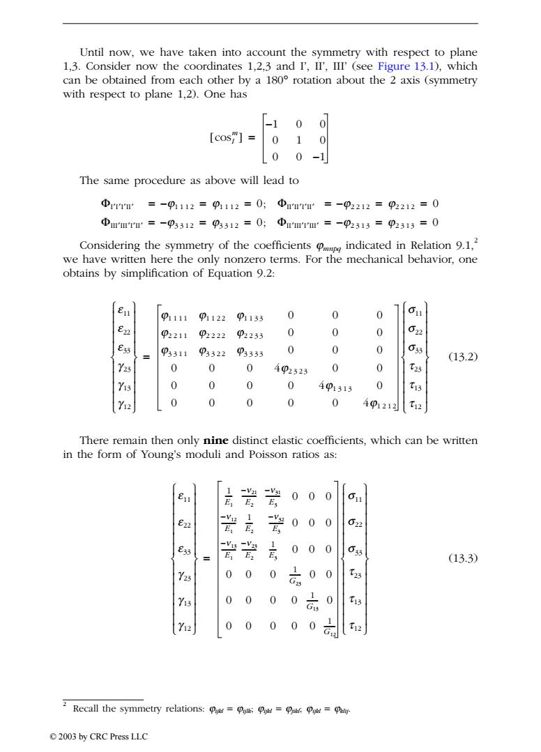
Until now,we have taken into account the symmetry with respect to plane 1,3.Consider now the coordinates 1,2,3 and I',II',III'(see Figure 13.1),which can be obtained from each other by a 180 rotation about the 2 axis (symmetry with respect to plane 1,2).One has -1 0 [cos"] 0 1 0 0 0-1 The same procedure as above will lead to Φ11=-p1112=p1112=0;Φ1m1rm=-p2212=p2212=0 Φmm1=-p3312=93312=0;①m1'm=-p2313=92313=0 Considering the symmetry of the coefficientsindicated in Relation9.1.2 we have written here the only nonzero terms.For the mechanical behavior,one obtains by simplification of Equation 9.2: e11 φ1111 φ1122 p1133 0 0 0 611 p2211 02222P2233 0 0 0 62 e38 03311 03322 03333 0 0 0 033 (13.2) Y23 0 0 0 492323 0 0 T23 Y13 0 0 0 0 401313 0 t 0 0 0 0 0 4φ1212 T12 There remain then only nine distinct elastic coefficients,which can be written in the form of Young's moduli and Poisson ratios as: e 1 岩 岩 00 0 011 e22 E 苦 00 0 022 e33 岩 E 言 000 033 (13.3) Y23 0 0 0 00 23 0 0 0 T13 0 0 0 0 T12 Recall the symmetry relations:===u 2003 by CRC Press LLC
Until now, we have taken into account the symmetry with respect to plane 1,3. Consider now the coordinates 1,2,3 and I’, II’, III’ (see Figure 13.1), which can be obtained from each other by a 180∞ rotation about the 2 axis (symmetry with respect to plane 1,2). One has The same procedure as above will lead to Considering the symmetry of the coefficients jmnpq indicated in Relation 9.1,2 we have written here the only nonzero terms. For the mechanical behavior, one obtains by simplification of Equation 9.2: (13.2) There remain then only nine distinct elastic coefficients, which can be written in the form of Young’s moduli and Poisson ratios as: (13.3) 2 Recall the symmetry relations: jijkl = jijlk; jijkl = jjikl; jijkl = jklij. cosI m [ ] –1 0 0 010 001– = FI¢I¢I¢II¢ = == = == –j1112 j1112 0; FII¢II¢I¢II¢ –j2212 j2212 0 FIII¢III¢I¢II¢ = == = == –j3312 j3312 0; FII¢III¢I¢III¢ –j2313 j2313 0 e 11 e 22 e 33 g 23 g 13 g 12 Ó ˛ Ô Ô Ô Ô Ô Ô Ô Ô Ì ˝ Ô Ô Ô Ô Ô Ô Ô Ô Ï ¸ j1111 j1122 j1133 000 j2211 j2222 j2233 000 j3311 j3322 j3333 000 0 0 04j2323 0 0 0 0 0 04j1313 0 0 0 0 0 04j1212 s11 s22 s33 t 23 t 13 t 12 Ó ˛ Ô Ô Ô Ô Ô Ô Ô Ô Ì ˝ Ô Ô Ô Ô Ô Ô Ô Ô Ï ¸ = e 11 e 22 e 33 g 23 g 13 g 12 Ó ˛ Ô Ô Ô Ô Ô Ô Ô Ô Ô Ô Ô Ô Ì ˝ Ô Ô Ô Ô Ô Ô Ô Ô Ô Ô Ô Ô Ï ¸ 1 E1 ---- –n21 E2 --------- –n31 E3 --------- 000 –n12 E1 --------- 1 E2 ---- –n32 E3 --------- 000 –n13 E1 --------- –n23 E2 --------- 1 E3 ---- 000 00 0 1 G23 ------- 0 0 00 00 1 G13 ------- 0 00 0 00 1 G12 ------- s11 s22 s33 t 23 t 13 t 12 Ó ˛ Ô Ô Ô Ô Ô Ô Ô Ô Ô Ô Ô Ô Ì ˝ Ô Ô Ô Ô Ô Ô Ô Ô Ô Ô Ô Ô Ï ¸ = TX846_Frame_C13 Page 261 Monday, November 18, 2002 12:29 PM © 2003 by CRC Press LLC
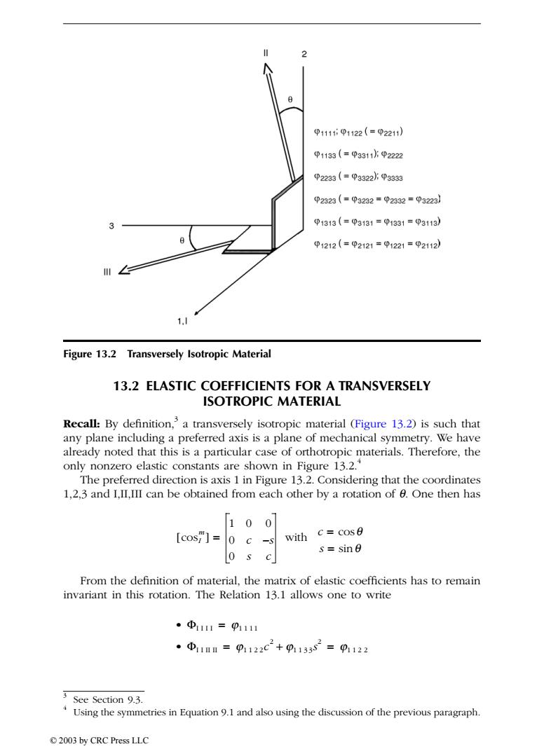
01111i01122(=02211) 01133(=93311水92222 02233(=93322i93333 02323(=93232=02332=p3223】 01313(=p3131=01331=03113) 01212(=02121=01221=02112) 1.l Figure 13.2 Transversely Isotropic Material 13.2 ELASTIC COEFFICIENTS FOR A TRANSVERSELY ISOTROPIC MATERIAL Recall:By definition,a transversely isotropic material (Figure 13.2)is such that any plane including a preferred axis is a plane of mechanical symmetry.We have already noted that this is a particular case of orthotropic materials.Therefore,the only nonzero elastic constants are shown in Figure 13.2. The preferred direction is axis 1 in Figure 13.2.Considering that the coordinates 1,2,3 and I,II,III can be obtained from each other by a rotation of 0.One then has [10 [cosT]= -S with c=cos0 s=sine 0 s From the definition of material,the matrix of elastic coefficients has to remain invariant in this rotation.The Relation 13.1 allows one to write 。Φ1111=p111 ·中1mm=91122c2+91332=91122 3 See Section 9.3. Using the symmetries in Equation 9.1 and also using the discussion of the previous paragraph. 2003 by CRC Press LLC
13.2 ELASTIC COEFFICIENTS FOR A TRANSVERSELY ISOTROPIC MATERIAL Recall: By definition,3 a transversely isotropic material (Figure 13.2) is such that any plane including a preferred axis is a plane of mechanical symmetry. We have already noted that this is a particular case of orthotropic materials. Therefore, the only nonzero elastic constants are shown in Figure 13.2. 4 The preferred direction is axis 1 in Figure 13.2. Considering that the coordinates 1,2,3 and I,II,III can be obtained from each other by a rotation of q. One then has From the definition of material, the matrix of elastic coefficients has to remain invariant in this rotation. The Relation 13.1 allows one to write Figure 13.2 Transversely Isotropic Material 3 See Section 9.3. 4 Using the symmetries in Equation 9.1 and also using the discussion of the previous paragraph. cosI m [ ] 10 0 0 c s – 0 s c = with c = cosq s = sinq • FI I I I = j1111 • FI I II II j1122c 2 j1133s 2 = = + j1122 TX846_Frame_C13 Page 262 Monday, November 18, 2002 12:29 PM © 2003 by CRC Press LLC