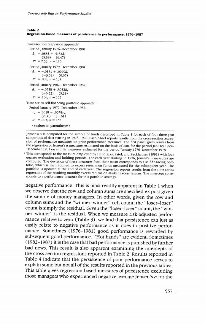
Survivorsbip Bias in Performance Studies Table 2 Regression-based measures of persistence in performance,1976-1987 Cross-section regression approach' Period January 1976-December 1981: a2=,0885+.4134a1 (5.38)(6.47) R2=2.53;n=126 Period January 1979-December 1984: c1■-.0831+.0070a, (-3.69)(0.07) R2=.000:n=134 Period January 1982-December 1987: a=-.0753+.3052a, (-6.53)(5.28) R2=.156:n=153 Time-series self-financing portfolio approach? Period January 1977-December 1987: m=0018-.0078r (2.88)(-.61) 2=.003;n=132 (t-values in parentheses) Jensen's a is computed for the sample of funds described in Table 1 for each of four three-year subperiods of data starting in 1976-1978.Each panel reports results from the cross-section regres sion of performance measures on prior performance measures.The first panel gives results from the regression of Jensen's a measures estimated on the basis of data for the period January 1979- December 1981 on similar measures estimated for the period January 1976-December 1978. This corresponds to the measure employed by Hendricks,Patel,and Zeckhauser (1991)with four quarter evaluation and holding periods.For each year starting in 1976,Jensen's a measures are computed.The deviation of these measures from their mean corresponds to a self financing port- folio,which is then applied to excess returns on funds measured for the subsequent year.The portfolio is updated at the end of each year.The regression reports results from the time-series regression of the resulting monthly excess returns on market excess returns.The intercept corre- sponds to a performance measure for this portfolio strategy. negative performance.This is most readily apparent in Table 1 when we observe that the row and column sums are specified ex post given the sample of money managers.In other words,given the row and column sums and the"winner-winner"cell count,the"loser-loser" count is simply the residual.Given the "loser-loser'count,the "win- ner-winner"is the residual.When we measure risk-adjusted perfor- mance relative to zero (Table 3),we find that persistence can just as easily relate to negative performance as it does to positive perfor- mance.Sometimes (1976-1981)good performance is rewarded by subsequent good performance."Hot hands"are evident.Sometimes (1982-1987)it is the case that bad performance is punished by further bad news.This result is also apparent examining the intercepts of the cross-section regressions reported in Table 2.Results reported in Table 4 indicate that the persistence of poor performance serves to explain some but not all of the results reported in the previous tables. This table gives regression-based measures of persistence excluding those managers who experienced negative average Jensen's a for the 5571
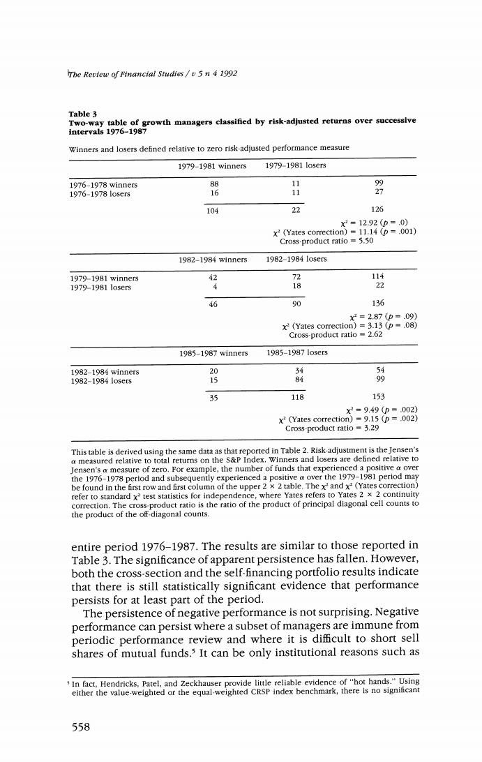
The Review of Financial Studies /v 5 n 4 1992 Table 3 Two-way table of growth managers classified by risk-adjusted returns over successive intervals 1976-1987 Winners and losers defined relative to zero risk-adjusted performance measure 1979-1981 winners 1979-19811o5ers 1976-1978 winner5 88 11 1976-1978lo5ers 16 11 27 104 22 126 x2=12.92(p=.0) x2 (Yates correction)=11.14 (p=.001) Cross-product ratio =5.50 1982-1984 winners 1982-19841o5er5 1979-1981 winners 2 72 114 1979-1981o5ers 18 22 46 90 136 xX2=2.87(p-.09) x2(Yates correction)=3.13 (p=.08) Cross-product ratio 2.62 1985-1987 winners 1985-19871osr5 1982-1984 winners 20 4 河 1982-19841o5er5 15 84 35 118 153 x2=9.49(p=.002) x2 (Yates correction)=9.15(p=.002) Cross-product ratio -3.29 This table is derived using the same data as that reported in Table 2.Risk-adjustment is the Jensen's a measured relative to total returns on the S&P Index.Winners and losers are defined relative to Jensen's a measure of zero.For example,the number of funds that experienced a positive a over the 1976-1978 period and subsequently experienced a positive a over the 1979-1981 period may be found in the first row and first column of the upper 2 x 2 table.The x'and x2(Yates correction) refer to standard x'test statistics for independence,where Yates refers to Yates 2 x 2 continuity correction.The cross-product ratio is the ratio of the product of principal diagonal cell counts to the product of the off-diagonal counts. entire period 1976-1987.The results are similar to those reported in Table 3.The significance of apparent persistence has fallen.However, both the cross-section and the self-financing portfolio results indicate that there is still statistically significant evidence that performance persists for at least part of the period. The persistence of negative performance is not surprising.Negative performance can persist where a subset of managers are immune from periodic performance review and where it is difficult to short sell shares of mutual funds.3 It can be only institutional reasons such as In fact,Hendricks,Patel,and Zeckhauser provide little reliable evidence of"hot hands."Using either the value-weighted or the equal-weighted CRSP index benchmark,there is no significant 558
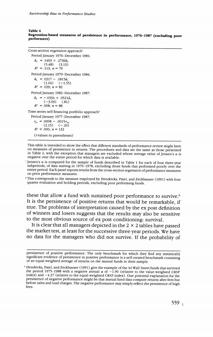
Survivorsbip Bias in Performance Studies Table 4 Regression-based measures of persistence in performance,1976-1987(excluding poor performers) Cross-section regression approach' Period January 1976-December 1981: 2=.1463+.2736à1 (5.48)(3.13) R2=.113;n=79 Period January 1979-December 1984: a■.0317-.18158 (1.04)(-1.55) 2=.029:n=82 Period January 1982-December 1987: 3=-.0334+.0521a (-3.09)(.81) R2=.008:n=88 Time-series self-financing portfolio approach? Period January 1977-December 1987: rw=.0008.-,0015rm (2.15)(-.20) 2=.000:n=132 (t-values in parentheses) This table is intended to show the effect that different standards of performance review might have on measures of persistence in returns.The procedures and data are the same as those presented in Table 2,with the exception that managers are excluded whose average value of Jensen's a is negative over the entire period for which data is available. "Jensen's a is computed for the sample of funds described in Table 1 for each of four three-year subperiods,of data starting in 1976-1978,excluding those funds that performed poorly over the entire period.Each panel reports results from the cross-section regression of performance measures on prior performance measures. This corresponds to the measure employed by Hendricks,Patel,and Zeckhauser (1991)with four quarter evaluation and holding periods,excluding poor performing funds. these that allow a fund with sustained poor performance to survive.6 It is the persistence of positive returns that would be remarkable,if true.The problems of interpretation caused by the ex post definition of winners and losers suggests that the results may also be sensitive to the most obvious source of ex post conditioning:survival. It is clear that all managers depicted in the 2 x 2 tables have passed the market test,at least for the successive three-year periods.We have no data for the managers who did not survive.If the probability of persistence of positive performance.The only benchmark for which they find any statistically significant evidence of persistence in positive performance is a self-created benchmark consisting of an equal-weighted average of returns on the mutual funds in their sample. Hendricks,Patel,and Zeckhauser(1991)give the example of the 44 Wall Street funds that survived the period 1975-1988 with a negative annual a of -1.90 (relative to the value-weighted CRSP index)and -4.27 (relative to the equal-weighted CRSP index).One potential explanation for the persistence of negative performance might be that mutual fund data compute returns after fees but before sales and load charges.The negative performance may simply reflect the persistence of high fees. 5591
Tbe Review of Financial Studtes/v 5 n 4 1992 survival depends on past performance to date,we might expect that the set of managers who survive will have a higher ex post return than those who did not survive.Managers who take on significant risk and lose may also have a low probability of survival.This observation suggests that past performance numbers are biased by survivorship; we only see the track record of those managers who have survived. This does not suggest,however,that performance persists.If anything, it suggests the reverse.If survival depends on cumulative perfor- mance,a manager who does well in one period does not have to do so well in the next period in order to survive.Certainly,this survi- vorship argument cannot explain results suggested by Table 1.More. over,there is a general perception that the survivorship bias effect cannot be very substantial.In a recent study,Grinblatt and Titman (1989)report that the survivorship effect accounts for only about 0.1 to 0.4 percent return per year measured on a risk-adjusted basis before transaction costs and fees.We shall see that the survivorship bias in mean excess returns is small in magnitude relative to a more subtle, yet surprisingly powerful,survival bias that implies persistence in performance. A manager who takes on a great deal of risk will have a high prob- ability of failure.However,if he or she survives,the probability is that this manager took a large bet and won.High returns persist.If they do not persist,we would not see this high-risk manager in our sample.7 Note that this is a total risk effect;risk-adjustment using B or other measure of nonidiosyncratic risk may not fully correct for it. To illustrate this effect,observe in Table 3 that the additional 10 firms that come into the database in 1979-1981 are all ex post successful. The average value of residual risk (0.0323)for the new entrants is significantly greater than that of the population of managers(0.0242), with a t-value of 2.02.The new entrants who survived took on more risk and were successful. The magnitude of the persistence will depend on the precise way in which survivorship depends on past performance and whether there is any strategic risk management response on the part of sur- viving money managers.8 The intent is to show that the apparent Hendricks,Patel,and Zeckhauser (1991)argue that because fund data is eliminated from their database as the fund ceases to exist or is merged into other funds,their sample is free of survivorship bias effects.However,all funds considered at each evaluation point survived at least until the end of an evaluation period that could extend from one quarter to two years.They are excluded from the analysis subsequent to the evaluation period.The numerical example given in Section 2 of this article matches this experimental design,and provides a counterexample to a presumption of freedom from survivorship bias effects.The results of such a study would be free of survival bias only if it can be established that the probability of termination or elimination from the sample is unrelated to performance.However,Hendricks,Patel,and Zeckhauser indicate (note 5)that,in fact,funds that go under do quite poorly in the quarter of demise. .We show in the Appendix that the effect is mitigated somewhat where cumulative performance 560
Survivorsbip Bias in Performance Studies persistence of performance documented in Tables 1 and 2 is not necessarily any indication of skill among surviving managers. To the extent that survivorship depends on past returns,ranking managers who survive by realized returns may induce an apparent persistence in performance.Survivorship implies that managers will be selected according to total risk.One way of explaining the Table 1 results is to observe that the set of managers studied represent a heterogeneous mix of management styles.Each management style is characterized by a certain vector of risk attributes.By examining the survivors,we are really only looking at those styles that were ex post successful.It may appear that one resolution of this problem is to concentrate on only one defined management style.There are two problems with this approach.In the first instance,we have to be careful to define the style sufficiently broadly that there are more than a few managers represented.In the second instance,we may exac- erbate the effect if our definition of manager style is synonymous with taking high total risk positions. We only observe the performance of managers who survive per. formance evaluations.The purpose of this article is to examine the extent to which this fact is sufficient to explain the magnitude of persistence we seem to see in the data.In Section 1,we examine the relationship between total risk differentials and survivorship-induced persistence in performance.In Section 2,we present some numerical results that show that a very small survivorship effect is sufficient to generate a strong and significant appearance of dependence in serial returns.We conclude in Section 3. 1.Relationship between Volatility and Returns Induced by Survivorship There are many possible quite complex sample selection rules.We will look at the implications of one class of these rules.Our purpose in this section is to demonstrate that sample survivorship bias is a force that can lead to persistence in performance rankings.For sim- plicity,assume all distributions are atomless.Our tool is the following lemma. rather than one-period performance is used as a survival criterion.The analysis of a strategic response is beyond the scope of this article.A possible strategic response is for surviving managers who are subject to the same survival criterion to converge in residual risk characteristics.The results in the next section require only that the ranking of managers by residual risk be constant.This kind of strategic response would also tend to mitigate the effect.This analysis is complicated by the fact that survival criteria are not necessarily the same for all managers. 5611